Lecture 5 Bayesian Inference
5.1 Overview
This lecture provides an introduction to Bayesian inference, the second major approach to statistical inference alongside likelihood-based inference. We start with the motivation for Bayesian Inference which arises from another philosophical perspective on the parameter of interest which states that it comes from a random distribution. By referring to Bayes’ Theorem we explain how the posterior distribution of the parameter is linked to three key components: the likelihood, the prior, and the marginal model. We then provide an example of such an bayesian approach. Finally, we present different types of prior distributions for the parameter of interest.
5.2 Reminder: Likelihood Inference
In likelihood inference, we have redefined the density as the likelihood: \[L_x(\theta) = \prod^n_{i=1}f(x_i | \theta)= p(x|\theta) = P_{\theta}(X=x) \] This means our objective function is the likelihood of the observed random data given the fixed parameter \(\theta\). To estimate the true population parameter \(\theta\), we maximize the likelihood with respect to \(\theta\): \[ \hat{\theta}_{ML} = \underset{\theta}{\operatorname{argmax}} L_x(\theta) \]
5.3 Philosophical Consideration: Parameter Distribution
Up to now we have assumed that only the data comes from a random distribution \(D\) while parameter(s) \(\theta\) are fixed: \[ X \sim D(\theta) \quad \text{where} \quad \theta = \text{const.} \] However, by using a likelihood it is only possible to infer the insecurity of the estimation but not on the distribution of the parameter itself.
Bayesian statistics builds upon the question whether a parameter can be fixed or if it is random anyway. It assumes that actually the data \(X\) is the observed and thus fixed size while the parameter it is actually the parameter \(\theta \in \mathbb{R}\) self has a random distribution \(D\) with parameter(s) \(\xi\): \(\theta \sim D(\xi)\). That leads to our target size now being \(p(\theta|X)\). This is called the posterior distribution of \(\theta\) since it is the distribution of the parameter after observing the data.
For the following sections we follow the bayesian approach and assume that the parameter of interest is not fixed but random.
5.4 Bayes’ Theorem
5.4.1 General Equation
Thomas Bayes’ Theorem provides a mathematical rule for inverting conditional probabilities. It is stated mthematically as the following equation: \[P(A|B) = \frac{P(B|A)P(A)}{P(B)}\] where \(A\) and \(B\) are events and \(P(B) \neq 0\).
- \(P(A|B)\) is the conditional probability of event \(A\) occurring given that \(B\) is true.
- \(P(B|A)\) is the conditional probability of event \(B\) occurring given that \(A\) is true.
- \(P(A)\) and \(P(B)\) are the probabilities of observing \(A\) and \(B\) respectively without any given conditions. They are known as the marginal probabilities.
The question now is: How can this be used for inference?
5.4.2 Application: Bayesian Inference
Substituting the target distribution \(p(\theta|X)\) into the left-hand side of Bayes’ Theorem yields the following equation: \[ p(\theta|X) = \frac{p(X|\theta)p(\theta)}{p(X)} \] where
- \(p(\theta|X)\) is the posterior distribution of the random parameter given the data.
- \(p(X|\theta)\) is the likelihood of the data given the fixed parameter.
- \(p(\theta)\) is the prior probability of the parameter.
- \(p(X)\) is the marginal distribution of the data.
We can now reinterpret this fraction as a framework for updating probabilities based on new evidence. Since the denominator is fixed, it is called the normalizing constant and does not affect the mode of the posterior. Hence, it is often sufficient to consider only the numerator, as the equations are proportional: \[ p(\theta|X) \propto p(X|\theta)p(\theta) \]
In Bayesian inference we now search for the distribution of the parameter given the data \(p(\theta|X)\). For this purpose we only need the likelihood \(p(X|\theta)\) and the prior distribution \(p(\theta)\).
5.5 Practical Example
5.5.1 Setting
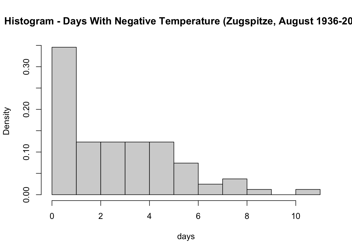
We assume that the data are realizations from a Poisson-distributed random variable \(X\). However, the rate parameter \(\lambda\) of this distribution is also assumed to be random. Given that it can only take positive values, suitable prior distributions include the Chi-Squared, Exponential, and Gamma distribution. Among these, the gamma distribution is often preferred, and we follow this choice:
- \(x_i \sim \Po(\lambda), i = 1,\ldots, n\)
- \(\lambda \sim \Ga(a_0, b_0)\)
As a result, the posterior distribution is proportional to: \[ p(\theta|X) \propto \underbrace{\prod^{n}_{i=1} \frac{\lambda^{x_i}}{x_i!}\exp{\left( -\lambda \right)}}_{\text{Likelihood: } p(X|\theta)} \underbrace{\frac{b_0^{a_0}}{\Gamma{(a_0)}}\lambda^{a_0-1}\exp{\left(-\lambda b_0\right)}}_{\text{Prior: }p(\theta)} \]
5.5.2 Result
The next step is to simplify the term and remove all parts that do not depend on \(\lambda\): \[ \begin{align} p(\theta|X) &\propto \lambda^{\sum^{n}_{i=1} x_i}\exp{\left(-n\lambda \right)} \lambda^{a_0-1}\exp{\left(-\lambda b_0\right)}\underbrace{\frac{b_0^{a_0}}{\Gamma{(a_0)}\prod^{n}_{i=1}x_i!}}_{\text{does not depend on } \lambda} \\ &\propto \lambda^{\left(a_0 + \sum^{n}_{i=1} x_i \right) -1}\exp{\left(-(n+b_0)\lambda \right)} \end{align} \] When having a closer look, the result has an identical kernel structure as the gamma prior. We conclude: \[ \lambda | x \sim \Ga\left(a_0 + \sum^{n}_{i=1} x_i, n+b_0\right) \]
The moments of a gamma distribution \(\Ga(\alpha, \beta)\) with parameters \(\alpha\) and \(\beta\) are given by \(E(X) = \frac{\alpha}{\beta}\) and \(\text{Var}{(X)} = \frac{\alpha}{\beta^2}\).
In our exemplary case, the posteriori mean is given by \[ \begin{align} E(\lambda|x) &= \frac{a_0 + \sum^{n}_{i=1} x_i}{n+b_0} \\ &= \frac{nb_0a_0 + nb_0\sum^{n}_{i=1} x_i}{nb_0(b_0+n)} \\ &= \frac{n}{b_0+n}\frac{\sum^{n}_{i=1} x_i}{n} + \frac{b_0}{b_0+n} \frac{a_0}{b_0} \\ &= \frac{n}{b_0+n} \hat{\lambda}_\text{ML} + \frac{b_0}{b_0+n} \hat{\lambda}_\text{prior} \end{align} \] and the posteriori variance is expressed as $$ \[\begin{align} \text{Var}{(\lambda|x)} &= \frac{a_0 + \sum^{n}_{i=1} x_i}{(n+b_0)^2} \\ &= \frac{\sum^{n}_{i=1} x_i}{(n+b_0)^2} + \frac{a_0}{(n+b_0)^2} \\ &= \frac{n^2}{(n+b_0)^2} \frac{\sum^{n}_{i=1} x_i}{n^2} + \frac{b_0^2}{(n+b_0)^2}\frac{a_0}{b_0^2} \\ &= \frac{n^2}{(n+b_0)^2} \text{Var}(\hat{\lambda}_{\text{ML}}) + \frac{b_0^2}{(n+b_0)^2}\text{Var}(\lambda_{\text{prior}}) \\ &= \left(\frac{n}{n+b_0}\right)^2 \text{Var}(\hat{\lambda}_{\text{ML}}) + \left(\frac{b_0}{n+b_0}\right)^2\text{Var}(\lambda_{\text{prior}}) \end{align}\] $$
5.5.3 Interpretation
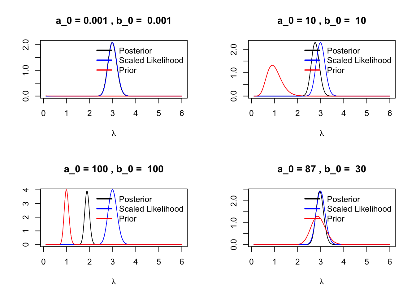
We observe that both the posterior mean and variance are weighted averages of the respective moments derived from the MLE and the prior distribution. Notably, a larger prior scale parameter \(b_0\) , which corresponds to a smaller prior variance, increases the prior’s influence. However, as the number of observations \(n\) increases, the likelihood’s influence becomes more dominant relative to the prior.
5.6 Interactive Shiny App
We have implemented this example in an interactive shiny app. Try out different values for the parameter values to see how prior distribution of the parameter is influenced is influenced by its two components, the likelihood and the prior distribution.
Click here for the full version of the ‘Introduction to Bayesian Statistics’ shiny app. It even includes a second example to play around with.
5.7 Types of Priors
A suitable prior distribution is one that matches the parameter space of the respective parameter. However, there are three special types of priors that are often used in practice:
- Conjugate priors
- Noninformative priors
- Jeffrey’s priors (not for now)
5.7.1 Conjugate Priors
A prior distribution \(p(\theta)\) is called conjugate prior for the likelihood \(L_x{\theta}\) if the posterior distribution \(p(\theta|x)\) is in the same distribution family.
- simpler inference
- detect by looking at the kernel of the distribution and the support of the prior
See above: gamma distribution conjugate with respect to \(\lambda\) for the poisson distribution
Probability Mass Function Poisson: \[f(x|\lambda) = \frac{\lambda^x}{x!} \mathrm{e}^{-\lambda}\]
Density Gamma: \[ f(x|\alpha,\beta) = \frac{\beta^\alpha}{\Gamma(\alpha)}x^{\alpha-1}\mathrm{e}^{-\beta x} \]