Lecture 4 Generalized Regression
4.1 Overview
In this lecture, we introduce Generalized Linear Models (GLMs), an extension of linear regression designed for situations where the dependent variable follows any distribution from the exponential family, expanding beyond the traditional normality assumption. Using an example with a Poisson-distributed response variable, we illustrate how these models are constructed and how the linear predictor is connected to the outcome. Additionally, we explore the properties of the exponential family, including its parameters, moments, and some examples. Finally, we present the general model equation for GLMs.
4.2 Introduction: Allbus Dataset
In this chapter, we introduce the Allbus (Allgemeine Bevölkerungsumfrage der Sozialwissenschaften) dataset, a large-scale survey that has been conducted since 1990/1991. It provides valuable insights into the attitudes, behaviors, and demographics of the German population. You can download the data on the official website of the GESIS.
For this lecture, we use a smaller subset of the Allbus dataset, focusing on data from the years 2014 and 2018. The following variables are contained in the dataset:
| Name | Description |
|---|---|
| respid | Unique identifier for each respondent |
| di07 | Migration background of the respondent (0 = No, 1 = Yes) |
| age | Age of the respondent |
| sex | Gender of the respondent (1 = Male, 2 = Female) |
| iscd11 | Highest level of education (ISCED 2011) |
| work | Employment status (1 = Employed, 2 = Unemployed, etc.) |
| eastwest | Region of residence (former East/West Germany) (1 = West, 2 = East) |
| german | German citizenship (0 = No, 1 = Yes) |
| feduc | Father’s highest level of education |
| meduc | Mother’s highest level of education |
| isei08 | Socioeconomic index of occupational status |
| worktime | Weekly working hours |
| tv | Daily television consumption (in minutes) |
Summary
allbus <- readRDS("./data/allbus_small.rds")
summary(allbus[,c(1:6)])
#>      respid            di07           sex
#>  Min.   :   1.0   Min.   :  183   male  :847
#>  1st Qu.: 899.5   1st Qu.: 1000   female:716
#>  Median :1755.0   Median : 1400
#>  Mean   :1768.3   Mean   : 1625
#>  3rd Qu.:2648.0   3rd Qu.: 2000
#>  Max.   :3476.0   Max.   :12600
#>
#>       age                                iscd11
#>  Min.   :18.00   upper secondary            :600
#>  1st Qu.:36.00   Masters or equiv           :414
#>  Median :47.00   short-cycle tertiary       :221
#>  Mean   :45.17   post secondary non-tertiary:146
#>  3rd Qu.:55.00   Bachelor's or equiv        : 71
#>  Max.   :78.00   lower secondary            : 60
#>                  (Other)                    : 51
#>            work
#>  full-time   :1245
#>  part-time   : 318
#>  side job    :   0
#>  not employed:   0
#>
#>
#>
summary(allbus[,c(7:13)])
#>  eastwest    german         feduc           meduc
#>  west:1111   yes:1469   Min.   :1.000   Min.   :1.000
#>  east: 452   no :  94   1st Qu.:2.000   1st Qu.:2.000
#>                         Median :2.000   Median :2.000
#>                         Mean   :2.855   Mean   :2.741
#>                         3rd Qu.:3.000   3rd Qu.:3.000
#>                         Max.   :6.000   Max.   :6.000
#>      isei08         worktime           tv
#>  Min.   :11.74   Min.   : 3.00   Min.   :  0.0
#>  1st Qu.:30.78   1st Qu.:35.00   1st Qu.: 60.0
#>  Median :54.55   Median :40.00   Median :120.0
#>  Mean   :51.44   Mean   :38.88   Mean   :111.4
#>  3rd Qu.:70.34   3rd Qu.:45.00   3rd Qu.:150.0
#>  Max.   :88.70   Max.   :98.00   Max.   :600.0
4.3 Modeling Approach: Linear Model
4.3.1 Model
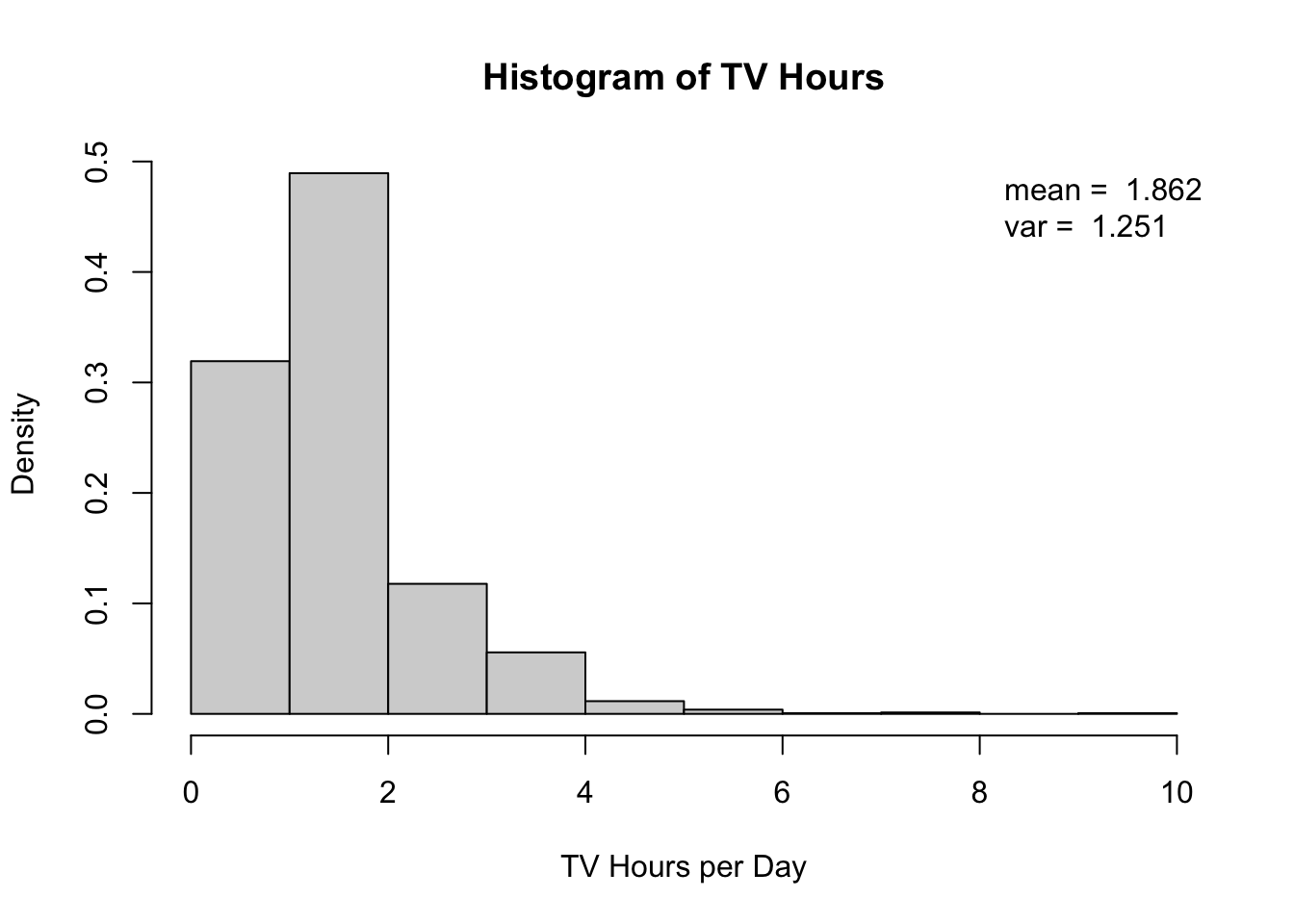
For the purpose of this lecture our variable of interest is the television consumption of the respondents. We transform the original variable tv so that the new variable, tv_hour, represents consumption in hours:
allbus$tv_hour <- round(allbus$tv/60)
hist(allbus$tv_hour, xlab="TV Hours per Day", main = "Histogram of TV Hours")
As independent variables we include worktime, sex, age, and loginc, which is the log of the income. The reason of the log-transformation lies in the negative skewness of the income. By taking the logarithm we obtain a more normally distributed covariate.
The equation of the linear model we want to estimate looks as follows:
\[ \text{tv_hour}_i = \beta_0 + \beta_1 \text{worktime}_i + \beta_2 \text{sex}_i + \beta_3 \text{age}_i + \beta_4 \text{loginc}_i + \varepsilon_i \]
4.3.2 Results
4.3.2.1 Regression
In the following you find the results after performing the regression in R:
allbus$loginc <- log(allbus$di07)
lm_tv <- lm(tv_hour ~ worktime + sex + age + loginc, data = allbus)
summary(lm_tv)
#>
#> Call:
#> lm(formula = tv_hour ~ worktime + sex + age + loginc, data = allbus)
#>
#> Residuals:
#>     Min      1Q  Median      3Q     Max
#> -2.3156 -0.7512  0.0553  0.4139  7.9919
#>
#> Coefficients:
#>              Estimate Std. Error t value Pr(>|t|)
#> (Intercept)  2.023719   0.399617   5.064 4.59e-07 ***
#> worktime    -0.001473   0.002814  -0.524   0.6007
#> sexfemale    0.026092   0.060876   0.429   0.6683
#> age          0.016262   0.002418   6.724 2.47e-11 ***
#> loginc      -0.117285   0.055773  -2.103   0.0356 *
#> ---
#> Signif. codes:
#> 0 '***' 0.001 '**' 0.01 '*' 0.05 '.' 0.1 ' ' 1
#>
#> Residual standard error: 1.103 on 1558 degrees of freedom
#> Multiple R-squared:  0.03022,    Adjusted R-squared:  0.02773
#> F-statistic: 12.14 on 4 and 1558 DF,  p-value: 1.016e-09
Examining the p-values, we find that the intercept, age, and loginc have statistically significant coefficients. Overall, the model explains approximately 3% of the variation in the response variable.
However, an analysis of the residuals reveals that the first and third quartiles are not symmetrically distributed around zero. This suggests that the residuals—and consequently, the response variable—do not follow a normal distribution. As a consequence, inference based on this model may not be reliable.
4.3.2.2 Prediction
We now plug the estimated model and different values for the covariates into the predict() command to make predictions for the daily hours of tv consumption. This function assumes a normally distributed response with the expectation coming from the linear model and the variance being constant:
\[
Y \sim \mathcal{N}(\mathbf{X} \boldsymbol{\beta}, \sigma^2), \quad Y \in \mathbb{R}
\]
predict(lm_tv,
        newdata = list(worktime = 0, sex = "female",
                       age = 56, loginc = 2))
#>        1
#> 2.725931

predict(lm_tv,
        newdata = list(worktime = 20, sex = "male",
                       age = 26, loginc = 4))
#>        1
#> 1.947933

predict(lm_tv,
        newdata = list(worktime = 140, sex = "male",
                       age = 16, loginc = 20))
#>          1
#> -0.2680488
For 56 year old women with zero hours work time per week and a log-income of 2, the expected daily TV consumption is 2.73 hours. Further, for 26 year old men with 20 weekly working hours and a log income of 4 we expect a TV consumption of 1.95 hours per day. However, when we take an out of sample example that is 16 years old, we expect -0.27 hours of watching TV per day which is not a meaningful value.
This already gives us a first guess that our model fails when it comes to predictions. We further examine this by comparing the kernel density estimate of the empirical TV hours data to the predicted values from our linear model.
plot(density(allbus$tv_hour), main = "Density of TV Hours")
lines(density(predict(lm_tv)), col = "grey")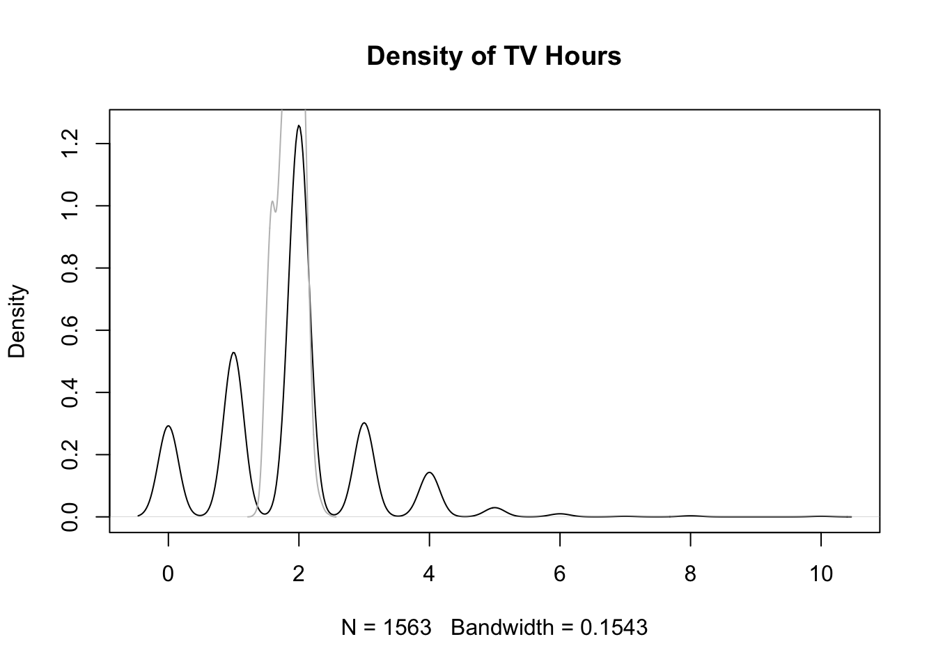 The real data distribution is multimodal with peaks every half hour while the predicted distribution is more concentrated with only one peak. It fails to capture the true variability, which highlights the mismatch between model and reality.
4.3.3 Problem of Linear Models
The problem of linear models is that the conditional distribution is fixed as a normal distribution with a fixed variance: \[Y_i \overset{iid}{\sim} N(\beta_0 + \beta_1 x_{i1} + \beta_2 x_{i2} + \cdots + \beta_p x_{ip} ,\sigma^2)\]
However, this assumption restricts the flexibility of the model, making it unsuitable for different types of variables or data distributions. To address this issue, the task is to adjust the conditional distribution to better fit the data.
4.4 Generalized Linear Models
4.4.1 Construction
For the construction of a generalized version of our linear regression model, we have three requirements. It should…
- … capture the domain of \(\mathbf{y}|\mathbf{X}\).
- … still keep the whole information of the covariates.
- … still use the closed form distributions (to be able to do inference).
4.4.2 Idea
The general idea is to use a conditional distribution that fits the experiment and estimate \(Y|X \sim D(d(x))\), where \(d(x)\) is some response function of the covariates.
To summarize, the three steps you have to think about are:
- Find a distribution that fits the response.
- Choose a response function \(h\) for the expected value of the response \(E(y) = h(f(x))\) or a link function \(g\) such that \(g(E(y)) = f(x) = \mathbf{X}\boldsymbol{\beta}\).
- Ensure that link and response functions are inversely related: \(g^{-1} = h\).
4.5 Modeling Approach: Generalized Linear Model
4.5.1 Distribution and Link Function
Since the data is discrete count data with values greater than or equal to zero we propose modeling it using the Poisson distribution. Thus, we need a response function that makes the linear regression equation positive: \(h(f(x)) > 0\). Potential choices for such a function include the absolute value, the square, or the exponential function, with the latter being the standard choice: \[\hat{y}_{Po} = \exp(\hat{\beta_0} + \hat{\beta_1}x_1+\dots)\] or in the case of our example \[\widehat{tv\_hour_i} = \exp(\hat{\beta_0} + \hat{\beta_1}worktime_i + \hat{\beta_2}sex_i + \hat{\beta_3}age_i + \hat{\beta_4}loginc_i)\]
4.5.2 Results
To estimate this model we use the glm() function in R with option family = "poisson":
glm_tv <- glm(tv_hour ~ worktime + sex + age + loginc,
              family = "poisson", data = allbus)
summary(glm_tv)
#>
#> Call:
#> glm(formula = tv_hour ~ worktime + sex + age + loginc, family = "poisson",
#>     data = allbus)
#>
#> Coefficients:
#>               Estimate Std. Error z value Pr(>|z|)
#> (Intercept)  0.7004645  0.2646700   2.647  0.00813 **
#> worktime    -0.0007592  0.0018572  -0.409  0.68270
#> sexfemale    0.0138623  0.0405453   0.342  0.73243
#> age          0.0088624  0.0016317   5.431 5.59e-08 ***
#> loginc      -0.0636080  0.0369873  -1.720  0.08548 .
#> ---
#> Signif. codes:
#> 0 '***' 0.001 '**' 0.01 '*' 0.05 '.' 0.1 ' ' 1
#>
#> (Dispersion parameter for poisson family taken to be 1)
#>
#>     Null deviance: 1239.9  on 1562  degrees of freedom
#> Residual deviance: 1207.9  on 1558  degrees of freedom
#> AIC: 4794.5
#>
#> Number of Fisher Scoring iterations: 5Derivation
We have a simple regression equation: \[ \hat{y} = \exp{(\hat{\beta}_0+\hat{\beta}_1x_1+\hat{\beta}_2x_2+\hat{\beta}_3x_3+\hat{\beta}_4x_4)} \] Increasing, for instance, the first covariate by one unit leads to the following estimation: \[ \begin{aligned} \hat{\tilde{y}} &= \exp{(\hat{\beta}_0+\hat{\beta}_1(x_1+1)+\hat{\beta}_2x_2+\hat{\beta}_3x_3+\hat{\beta}_4x_4)} \\ &= \exp{(\hat{\beta}_0+\hat{\beta}_1x_1+\hat{\beta}_2x_2+\hat{\beta}_3x_3+\hat{\beta}_4x_4)}*\exp{(\hat{\beta}_3)} \\ &= \hat{y}*exp{(\hat{\beta}_3)} \end{aligned} \]
4.6 Exponential Family
4.6.1 Probability Density Function
Generalized Linear Models, as implemented above, are possible for a certain class of distributions that belong to the (single-parameter) exponential family. A distribution of random variable \(Y\) belongs to the single-parameter exponential family (\(Y \sim EF\)) if the density can be written as \[ f_Y(y|\theta) = \exp \left(\frac{y\theta - b(\theta)}{\phi} \omega + c(y, \phi, \omega)\right) \]
Remarks:
- The parameter \(\theta\) is called the canonical parameter.
- The function \(b(\theta)\) has to be constructed such that \(f(y|\theta)\) can be normed and the derivations \(b'(\theta)\) and \(b''(\theta)\) exist.
- The function \(c(y, \phi, \omega)\) does not rely on \(\theta\).
- The parameter \(\phi\) is called the dispersion parameter.
- \(\omega\) is known (usually some kind of weight).
4.6.2 Moments
It can be shown that \(\mathbb{E}[y] = b'(\theta)\) and \(\text{Var}[y] = \frac{\phi}{\omega}b''(\theta)\).
Derivation: Expected Value
First, taking the first derivative of the exponential family distribution function w.r.t. \(\theta\) yields: \[ \frac{d}{d\theta} f_Y(y|\theta) = f_Y(y|\theta) * \left(\frac{y - b'(\theta)}{\phi} \omega \right) \] Now, we can integrate out \(y\) on both sides of the equation. By following Leibniz’s rule, we obtain for the left-hand side: \[ \int \frac{d}{d\theta} f_Y(y|\theta) \hspace{0.25em}dy = \frac{d}{d\theta} \underbrace{\int f_Y(y|\theta)\hspace{0.25em}dy}_{=1} = 0 \] For the right-hand side: \[ \int f_Y(y|\theta) * \left(\frac{y - b'(\theta)}{\phi} \omega \right) dy \\ = \frac{\omega}{\phi} \int f_Y(y|\theta) * \left(y - b'(\theta)\right) dy \\ = \frac{\omega}{\phi} \left( \int f_Y(y|\theta) * y \enspace dy - \int f_Y(y|\theta) * b'(\theta) \hspace{0.25em} dy \right) \\ = \frac{\omega}{\phi} \left(\mathbb{E}[y] - b'(\theta ) \underbrace{\int f_Y(y|\theta) \hspace{0.25em}dy}_{=1} \right) \\ = \frac{\omega}{\phi} \left(\mathbb{E}[y] - b'(\theta )\right) \] Finally, we can find the value of the expectation by equating both sides of the equation: \[ 0 = \frac{\omega}{\phi} \left(\mathbb{E}[y] - b'(\theta )\right) \\ \Leftrightarrow \mathbb{E}[y] = b'(\theta) \quad \text{q.e.d.} \]
Derivation: Variance
The first step is to take the second derivative of the exponential family distribution function w.r.t. \(\theta\): \[ \begin{align} \frac{d^2}{d\theta^2} f_Y(y|\theta) &= \frac{d}{d\theta} \left[ f_Y(y|\theta) * \left(\frac{y - b'(\theta)}{\phi} \omega \right) \right] \\ &= f_Y(y|\theta) * \frac{- b''(\theta)}{\phi} \omega + f_Y(y|\theta) * \left(\frac{y - b'(\theta)}{\phi} \omega \right) * \left(\frac{y - b'(\theta)}{\phi} \omega \right) \\ &= f_Y(y|\theta) * \left[ \left(y - b'(\theta)\right)^2 \frac{\omega^2}{\phi^2} - \frac{b''(\theta)}{\phi} \omega \right] \end{align} \]
Now we integrate out \(y\) on both sides of the equation. Firstly, applying Leibniz’s rule lets us simplify the left-hand side as: \[ \int \frac{d^2}{d\theta^2} f_Y(y|\theta)\hspace{0.25em} dy = \frac{d^2}{d\theta^2} \underbrace{\int f_Y(y|\theta)}_{=1}\hspace{0.25em} dy = 0 \] Secondly, for the right-hand side we obtain the following result: \[ \int f_Y(y|\theta) * \left[ \left(y - b'(\theta)\right)^2 \frac{\omega^2}{\phi^2} - \frac{b''(\theta)}{\phi} \omega \right]\hspace{0.25em} dy \\ = \int f_Y(y|\theta) * \left(y - b'(\theta)\right)^2 \frac{\omega^2}{\phi^2} \hspace{0.25em} dy - \int f_Y(y|\theta) * \frac{b''(\theta)}{\phi} \omega \hspace{0.25em} dy \\ = \frac{\omega^2}{\phi^2} \int f_Y(y|\theta) * \left(y - b'(\theta)\right)^2 \hspace{0.25em} dy - \frac{b''(\theta)}{\phi} \omega \underbrace{\int f_Y(y|\theta)\hspace{0.25em} dy}_{=1} \\ = \frac{\omega^2}{\phi^2} \text{Var}[y] - \frac{b''(\theta)}{\phi} \omega \] Equating the results for both sides gives us: \[ 0 = \frac{\omega^2}{\phi^2} Var[y] - \frac{b''(\theta)}{\phi} \omega \\ \Leftrightarrow \text{Var}[y] = \frac{\phi}{\omega}b''(\theta) \quad \text{q.e.d.} \]
4.6.3 Examples
Some exemplary distributions that belong to the exponential family are the (Inverse) Gaussian, Exponential, (Inverse) Gamma, Beta, Bernoulli, (Negative) Binomial, and the Poisson distribution.
Example: Gaussian Distribution
The probability density function of the normal distribution is defined as: \[ f_Y(y \mid \mu, \sigma) = \frac{1}{\sqrt{2\pi\sigma^2}} \exp\left( -\frac{(y - \mu)^2}{2\sigma^2} \right) \] We assume \(\sigma^2\) as constant and \(\mu\) as being the only unknown parameter. Now, putting everything into the exponential term yields: \[ f_Y(y \mid \mu) = \exp\left( -\frac{(y - \mu)^2}{2\sigma^2} + \log{\frac{1}{\sqrt{2\pi\sigma^2}}}\right) \]
Next, multiplying out the square in the numerator yields: \[ f_Y(y \mid \mu) = \exp\left( -\frac{y^2 - 2y\mu + \mu^2}{2\sigma^2} + \log{\frac{1}{\sqrt{2\pi\sigma^2}}}\right) \] Rearranging and simplifying terms gives us: \[ f_Y(y \mid \mu) = \exp\left(\frac{y\mu - \frac{1}{2}\mu^2}{\sigma^2} - \frac{y^2}{2\sigma^2} + \log{\frac{1}{\sqrt{2\pi\sigma^2}}}\right) \] This equation is already sufficient to prove that the Gaussian distribution comes from the exponential family with parameters:
- \(\theta = \mu\)
- \(b(\theta) = \frac{1}{2}\mu^2\), \(b'(\mu) = \mu\), \(b''(\mu) = \sigma^2\)
- \(\phi = \sigma^2\)
- \(\omega = 1\)
- \(c(y, \phi, \omega) = - \frac{y^2}{2\sigma^2} + \log{\frac{1}{\sqrt{2\pi\sigma^2}}}\)
Example: Poisson Distribution
The probability density function of the poisson distribution is defined as: \[ f_Y(y \mid \lambda) = \frac{\exp(-\lambda) \lambda^y}{y!} \] Putting everything into the exponential term and rearranging yields: \[ f_Y(y \mid \lambda) = \exp\left(y\log\lambda -\lambda - \log{y!}\right) \] This equation is already sufficient to prove that the Gaussian distribution comes from the exponential family with parameters:
- \(\theta = \log\lambda\)
- \(b(\theta) = \exp(\log\lambda) =\lambda\), \(b'(\theta) = \lambda\), \(b''(\theta) = \lambda\)
- \(\phi = 1\)
- \(\omega = 1\)
- \(c(y, \phi, \omega) = - \log{y!}\)
4.7 General Definition
For all distributions in the single-parametric exponential family, we can define the general model class of Generalized Linear Models (GLM):
- Distributional Assumption: \[y_i | \boldsymbol{x}_i\ \stackrel{iid}{\sim} \text{EF} \quad \text{with} \quad \mu_i = \mathbb{E}(y_i | \boldsymbol{x}_i)\]
- Structural Assumption: The expectation \(\mu_i\) is linked to the linear predictor \(\eta_i\) by a (reversible and twice differential) response function \(h\): \[\mu_i = h(\eta_i) \quad \text{with} \quad \eta_i = \boldsymbol{x}_i^\top \boldsymbol{\beta} = \beta_0 + \beta_1 x_{i1} + \ldots + \beta_k x_{ik}\] This renders possible a unified theory for parameter estimation and hypothesis testing and a unified estimation framework in statistical programming.