Lecture 3 Linear Regression
3.1 Overview
In this lecture we will introduce linear regression. We will start with the simple linear regression and focus on the history, model assumptions, and properties of the least squares estimator. Finally, we will extend this model by adding more covariates to obtain a multiple linear regression and finally show that with likelihood estimation we obtain the same result as with OLS.
3.2 Simple Linear Regression
3.2.1 History on Linear Models
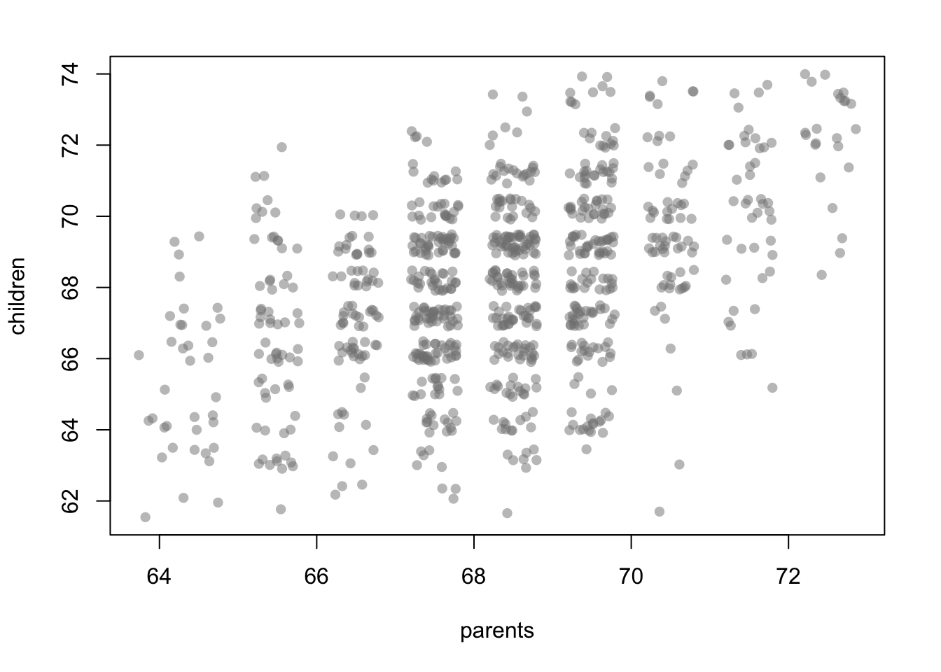 In the plot it can be observed that an extreme value in the heights of the parents does not automatically lead to an extreme value for the child. Instead, there is a tendency there is a tendency to “regress to” the (conditional) mean.
3.2.2 Regression Equation
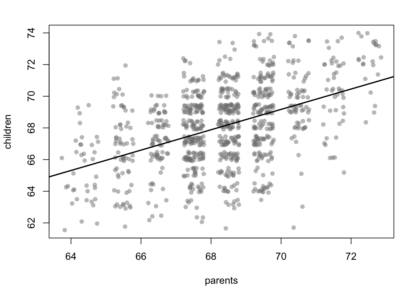
To capture this relationship between two variables, a simple linear line, representing this conditional mean of the data, can be used.
We explain a so-called response variable \(Y_i\) using a function \(f(x_i)\) to model an average relationship and \(\varepsilon_i\) as an residual (error term), which captures the unexplainable random noise. \[\begin{array}{lllll} Y_i & = & f(x_i) & + & \varepsilon_i \\ \mbox{response} & = & \mbox{average} & + & \mbox{error} \\ \mbox{variable} & & \mbox{relationship} & & \mbox{term} \\ \end{array}\]
There are many different options to model equation \(f(x_i)\). In our case with only one covariate, a simple linear line can be used to represent the conditional mean of the data. \[Y_i = \beta_0 + \beta_1 x_i + \varepsilon_i\] i.e. \[f(x_i) = \beta_0 + \beta_1 x_i\] where \(\beta_0\) is the intercept, \(\beta_1\) the slope coefficient, and \(x_i\) a single covariate. The challenge now is determining how to find the best estimates for \(\beta_0\) and \(\beta_1\) that accurately fit the data.
3.2.3 Concept: Least Squares Estimation
Carl Friedrich Gauss’s development of the method of least squares provided an elegant solution to this problem. The core idea is to minimize the sum of squared differences between the regression line and the observed data: \[ \left(\hat{\beta_0}, \hat{\beta_1} \right)^\top = \underset{\beta_0, \beta_1}{\operatorname{argmin}} \sum_{i=1}^n \left(Y_i - (\beta_0 + \beta_1 x_i) \right)^2 \quad \text{where} \quad Y_i - (\beta_0 + \beta_1 x_i) = \varepsilon_i \] Squaring the differences ensures that larger deviations are given more weight and eliminates the issue of residuals canceling each other out due to differing signs.
3.2.4 Application: Least Squares Estimation
For a better understanding we provide an interactive shiny application. The example used in the app focuses on the influence of speed in mph on the braking distance in feet. We mark the data points in blue and the regression line in red. Further, the plot shows three green squares that represent the squared residuals of three random observations. Summing up all of these squares yields the residual sum of squares \(SSR\) which is shown in the top left corner. You can move the sliders and observe how the red regression line adapts. Since this is the goal in OLS estimation, try to minimize the \(SSR\) to find the best fit.
Click here for the full version of the ‘Linear Regression’ shiny app.
3.2.5 Model Assumptions
The error terms are independently and identically distributed (iid) with \(E(\varepsilon_i) = 0\) and \(\mathop{\mathrm{Var}}(\varepsilon_i) = \sigma^2\) (homoscedastic variance).
For determining Test- and Confidence Intervals we additionally assume the error terms \(\varepsilon_i\) to be normally distributed, i.e. \(\varepsilon_i \sim N(0,\sigma^2)\).
Thus the resulting distribution of \(Y_i\) is
- \(E(Y_i) = E(\beta_0 + \beta_1 x_i + \varepsilon_i) = \beta_0 + \beta_1 x_i + E(\varepsilon_i) = \beta_0 + \beta_1 x_i,\)
- \(\mathop{\mathrm{Var}}(Y_i) = \mathop{\mathrm{Var}}(\beta_0 + \beta_1 x_i + \varepsilon_i) = \mathop{\mathrm{Var}}(\varepsilon_i) = \sigma^2,\) \[\Rightarrow Y_i \overset{iid}{\sim} N(\beta_0 + \beta_1 x_i,\sigma^2).\]
3.2.6 Result: Least Squares Estimator
The least squares estimators for the intercept and the slope are:
- \(\hat{\beta_1} = \frac{\sum_{i=1}^n (x_i - \bar{x})(y_i - \bar{y})}{\sum_{i=1}^n (x_i - \bar{x})^2}\)
- \(\hat{\beta_0} = \bar{y} - \beta_1 \bar{x}\)
Derivation
We start with the sum of squared residuals (SSR) for a simple linear regression model:
\[ SSR = \sum_{i=1}^n \left( y_i - (\beta_0 + \beta_1 x_i) \right)^2 \]
The goal is to minimize \(SSR\) with respect to \(\beta_0\) and \(\beta_1\). To do so, we take partial derivatives with respect to \(\beta_0\) and \(\beta_1\), and set them to zero:
-
Partial Derivative with Respect to \(\beta_0\): \[ \frac{\partial SSR}{\partial \beta_0} = -2 \sum_{i=1}^n \left( y_i - (\beta_0 + \beta_1 x_i) \right) = 0 \]
Simplify: \[ \sum_{i=1}^n y_i = n\beta_0 + \beta_1 \sum_{i=1}^n x_i \]
Rearrange to express the first equation: \[ \beta_0 n + \beta_1 \sum_{i=1}^n x_i = \sum_{i=1}^n y_i \tag{1} \]
-
Partial Derivative with Respect to \(\beta_1\): \[ \frac{\partial SSR}{\partial \beta_1} = -2 \sum_{i=1}^n x_i \left( y_i - (\beta_0 + \beta_1 x_i) \right) = 0 \]
Simplify: \[ \sum_{i=1}^n x_i y_i = \beta_0 \sum_{i=1}^n x_i + \beta_1 \sum_{i=1}^n x_i^2 \]
Rearrange to express the second equation: \[ \beta_0 \sum_{i=1}^n x_i + \beta_1 \sum_{i=1}^n x_i^2 = \sum_{i=1}^n x_i y_i \tag{2} \]
From equations (1) and (2), we now solve for \(\beta_0\) and \(\beta_1\):
Rewrite equation (1) for \(\beta_0\): \[ \beta_0 = \frac{1}{n} \left( \sum_{i=1}^n y_i - \beta_1 \sum_{i=1}^n x_i \right) \]
Substitute this expression for \(\beta_0\) into equation (2): \[ \frac{1}{n} \left( \sum_{i=1}^n y_i - \beta_1 \sum_{i=1}^n x_i \right) \sum_{i=1}^n x_i + \beta_1 \sum_{i=1}^n x_i^2 = \sum_{i=1}^n x_i y_i \]
-
Simplify to isolate \(\hat{\beta_1}\): \[ \beta_1 = \frac{\sum_{i=1}^n (x_i - \bar{x})(y_i - \bar{y})}{\sum_{i=1}^n (x_i - \bar{x})^2} \]
Where \(\bar{x} = \frac{1}{n} \sum_{i=1}^n x_i\) and \(\bar{y} = \frac{1}{n} \sum_{i=1}^n y_i\).
Use the value of \(\beta_1\) to compute \(\hat{\beta_0}\): \[ \beta_0 = \bar{y} - \beta_1 \bar{x} \]
3.2.7 Properties of the Least Squares Estimator
There are two important properties of the LS-estimator: unbiasedness and consistency.
Unbiased: The LS-estimator is unbiased, i.e. \[E(\hat{\beta}_0) = \beta_0, \qquad E(\hat{\beta}_1) = \beta_1.\]
Variance: \[\begin{aligned} \mathop{\mathrm{Var}}(\hat{\beta}_0) & = & \sigma^2 \displaystyle \frac{\sum\limits_{i=1}^{n} x_i^2}{n \sum\limits_{i=1}^{n} (x_i-\bar{x})^2}, \\ \mathop{\mathrm{Var}}(\hat{\beta}_1) & = & \displaystyle \frac{\sigma^2}{\sum\limits_{i=1}^{n} (x_i-\bar{x})^2}.\end{aligned}\]
If \(n \rightarrow \infty\) \[\sum\limits_{i=1}^{n} (x_i - \bar{x})^2 \rightarrow \infty\] holds, \(\hat{\beta}_0\) and \(\hat{\beta}_1\) are consistent as well since the variances decrease towards zero.
In the following we provide proofs for both conditions:
Proof: Unbiasedness
1. Estimator for \(\hat{\beta}_1\)
The formula for the slope estimator \(\hat{\beta}_1\) is:
\[\hat{\beta}_1 = \frac{\sum_{i=1}^n (x_i - \bar{x})(y_i - \bar{y})}{\sum_{i=1}^n (x_i - \bar{x})^2}\]
Substitute \(y_i = \beta_0 + \beta_1 x_i + \varepsilon_i\) and break into terms:
\[\hat{\beta}_1 = \frac{\sum_{i=1}^n (x_i - \bar{x}) \left(\beta_0 + \beta_1 x_i + \varepsilon_i - \bar{y}\right)}{\sum_{i=1}^n (x_i - \bar{x})^2} \\= \frac{\sum_{i=1}^n (x_i - \bar{x}) \left(\beta_0 - \bar{y}\right) + \sum_{i=1}^n (x_i - \bar{x}) \beta_1 x_i + \sum_{i=1}^n (x_i - \bar{x}) \varepsilon_i}{\sum_{i=1}^n (x_i - \bar{x})^2}\]
The first term simplifies because:
\[\sum_{i=1}^n (x_i - \bar{x}) = 0 \quad (\text{since } \bar{x} \text{ is the mean of } x_i)\]
For the second term:
\[\sum_{i=1}^n (x_i - \bar{x}) x_i = \sum_{i=1}^n (x_i - \bar{x}) (\bar{x} + (x_i - \bar{x})) = \sum_{i=1}^n (x_i - \bar{x})^2\]
So this term simplifies to:
\[\beta_1 \sum_{i=1}^n (x_i - \bar{x})^2\]
For the third term:
\[\sum_{i=1}^n (x_i - \bar{x}) \varepsilon_i\]
Since \(\varepsilon_i\) is iid random with \(\mathbb{E}[\varepsilon_i] = 0\), its expectation is:
\[\mathbb{E}\left[\sum_{i=1}^n (x_i - \bar{x}) \varepsilon_i\right] = 0\]
Thus, the expectation of \(\hat{\beta}1\) is:
\[\mathbb{E}\left[\hat{\beta}_1\right] = \frac{\beta_1 \sum_{i=1}^n (x_i - \bar{x})^2}{\sum_{i=1}^n (x_i - \bar{x})^2} = \beta_1.\]
2. Estimator for \(\hat{\beta}_0\)
The formula for the intercept estimator \(\hat{\beta}_0\) is:
\[\hat{\beta}_0 = \bar{y} - \hat{\beta}_1 \bar{x}\]
Substitute \(\bar{y} = \frac{1}{n} \sum_{i=1}^n y_i\) and \(y_i = \beta_0 + \beta_1 x_i + \varepsilon_i\):
\[\bar{y} = \frac{1}{n} \sum_{i=1}^n (\beta_0 + \beta_1 x_i + \varepsilon_i) = \beta_0 + \beta_1 \bar{x} + \bar{\varepsilon}\]
Here, \(\bar{\varepsilon} = \frac{1}{n} \sum_{i=1}^n \varepsilon_i\), and since \(\mathbb{E}[\varepsilon_i] = 0\), we have \(\mathbb{E}[\bar{\varepsilon}] = 0\)
Now substitute into \(\hat{\beta}_0\):
\[\hat{\beta}_0 = \bar{y} - \hat{\beta}_1 \bar{x} = (\beta_0 + \beta_1 \bar{x} + \bar{\varepsilon}) - \hat{\beta}_1 \bar{x}\]
Taking the expectation: \[\mathbb{E}\left[\hat{\beta}_0\right] = \beta_0 + \beta_1 \bar{x} - \mathbb{E}\left[\hat{\beta}_1\right] \bar{x}\]
From the previous result, \(\mathbb{E}\left[\hat{\beta}_1\right] = \beta_1\). Substituting:
\[\mathbb{E}\left[\hat{\beta}_0\right] = \beta_0 + \beta_1 \bar{x} - \beta_1 \bar{x} = \beta_0\]
Proof: Variance and Consistency
- Variance of \(\hat{\beta}_1\):
Using the definition of \(\hat{\beta}_1\):
\[\hat{\beta}_1 = \frac{\sum_{i=1}^n (x_i - \bar{x})(y_i-\bar{y})}{\sum_{i=1}^n (x_i - \bar{x})^2}\]
We can rewrite the numerator: \[\hat{\beta}_1 = \frac{\sum_{i=1}^n (x_i - \bar{x})(\beta_0 + \beta_1x_i+\varepsilon_i-\bar{\beta_0} - \bar{\beta_1}\bar{x} - \bar{\varepsilon})}{\sum_{i=1}^n (x_i - \bar{x})^2}\] Since the coefficients are constants, we can rewrite \(\bar{\beta_0} = \beta_0\) and \(\bar{\beta_1} = \beta_1\). Furthermore, by definition \(\bar{\varepsilon} = 0\). Hence, the numerator can be summarized as: \[\hat{\beta}_1 = \frac{\sum_{i=1}^n (x_i - \bar{x})(\beta_1(x_i-\bar{x})+\varepsilon_i)}{\sum_{i=1}^n (x_i - \bar{x})^2} \\ = \beta_1 + \frac{\sum_{i=1}^n (x_i - \bar{x})\varepsilon_i}{\sum_{i=1}^n (x_i - \bar{x})^2}\]
We take the variance: \[ \text{Var}(\hat{\beta_1}) = \text{Var}\left( \beta_1 + \frac{\sum_{i=1}^n (x_i - \bar{x})\varepsilon_i}{\sum_{i=1}^n (x_i - \bar{x})^2}\right) \] Since the coefficient \(\beta_1\) is assumed as fix, its (co-)variance is equal to zero:
\[\text{Var}(\hat{\beta}_1) = \text{Var}\left(\frac{\sum_{i=1}^n (x_i - \bar{x}) \varepsilon_i}{\sum_{i=1}^n (x_i - \bar{x})^2}\right)\]
The denominator \(\sum_{i=1}^n (x_i - \bar{x})^2\) is a constant, so we can pull it out by squaring:
\[\text{Var}(\hat{\beta}_1) = \frac{\text{Var}\left(\sum_{i=1}^n (x_i - \bar{x}) \varepsilon_i\right)}{\left(\sum_{i=1}^n (x_i - \bar{x})^2\right)^2}\] Now the only random part are the \(\varepsilon_i\), which are independent and identically distributed with \(\text{Var}(\varepsilon_i) = \sigma^2\). The variance of this weighted sum of independent variables is:
\[\text{Var}\left(\sum_{i=1}^n (x_i - \bar{x}) \varepsilon_i\right) = \sum_{i=1}^n (x_i - \bar{x})^2 \text{Var}(\varepsilon_i) \\ = \sigma^2 \sum_{i=1}^n (x_i - \bar{x})^2\]
Thus:
\[\text{Var}(\hat{\beta}_1) = \frac{\sigma^2 \sum_{i=1}^n (x_i - \bar{x})^2}{\left(\sum_{i=1}^n (x_i - \bar{x})^2\right)^2}\]
Simplify: \[\text{Var}(\hat{\beta}_1) = \frac{\sigma^2}{\sum_{i=1}^n (x_i - \bar{x})^2}\]
2. Variance of \(\hat{\beta}_0\):
Using \(\hat{\beta}_0 = \bar{y} - \hat{\beta}_1 \bar{x}\), the variance is:
\[\text{Var}(\hat{\beta}_0) = \text{Var}(\bar{y}) + \bar{x}^2 \text{Var}(\hat{\beta}_1) - 2\bar{x} \, \text{Cov}(\bar{y}, \hat{\beta}_1)\]
Variance of \(\bar{y}\): Since \(\bar{y} = \frac{1}{n} \sum_{i=1}^n y_i\) and \(y_i = \beta_0 + \beta_1 x_i + \varepsilon_i\), the variance of \(\bar{y}\) is:
\[\text{Var}(\bar{y}) = \frac{\sigma^2}{n}\]
Covariance of \(\bar{y}\) and \(\hat{\beta}_1\): We add this term since both \(\bar{y}\) and \(\hat{\beta}_1\) consist of the random variable \(\varepsilon_i\). However, the covariance \(\text{Cov}(\bar{y}, \hat{\beta}_1)\) is 0 because \(\bar{y}\) depends on the average of \(\varepsilon_i\), which is zero by definition. Further, \(\hat{\beta}_1\) depends on the deviations from \(\bar{x}\) (see above), which are orthogonal to \(\bar{y}\).
Combine terms: Substitute into the formula:
\[\text{Var}(\hat{\beta}_0) = \frac{\sigma^2}{n} + \bar{x}^2 \frac{\sigma^2}{\sum_{i=1}^n (x_i - \bar{x})^2}\]
Factor out \(\frac{\sigma^2}{\sum_{i=1}^n (x_i - \bar{x})^2}\):
\[\text{Var}(\hat{\beta}_0) = \frac{\sigma^2 \sum_{i=1}^n x_i^2}{n \sum_{i=1}^n (x_i - \bar{x})^2}\]
3. Consistency
Both terms tend towards zero when \(n \to \infty\):
For \(\text{Var}(\hat{\beta_1})\): \[ \lim_{n \to \infty} \frac{\sigma^2}{\sum_{i=1}^n (x_i - \bar{x})^2} = 0 \]
For \(\text{Var}(\hat{\beta_0})\): \[ \lim_{n \to \infty} \frac{\sigma^2 \sum_{i=1}^n x_i^2}{n \sum_{i=1}^n (x_i - \bar{x})^2} = 0 \]
Unless the \(x_i\)’s are constant (which they’re not in most cases), the sums in both denominators keeps increasing as you add more data points.
Hence, the estimators are asymptotically efficient.
3.3 Multiple Linear Regression
Until now we only considered models with one covariate \(X\). From now on consider \(p\) covariates \(X_1,\dots,X_p\) with observations \(x_{i1},\dots,x_{ip}\), \(i=1,\dots,n\). Extending the example from above, we could probably also be interested in the parents’ income or the diet of the children as influence factors of the height.
General model assumption: \[\begin{array}{lllll} Y_i & = & f(x_i) & + & \varepsilon_i \\ \mbox{response} & = & \mbox{average} & + & \mbox{error} \\ \mbox{variable} & & \mbox{relationship} & & \mbox{term} \\ \end{array}\]
From now we call this model just linear model.
3.3.1 Model Formulation
The formula of the linear regression model is as follows: \[Y_i = \beta_0 + \beta_1 x_{i1} + \beta_2 x_{i2} + \cdots + \beta_p x_{ip} + \varepsilon_i,\] i.e. \[f(x_{i1},\dots,x_{ip}) = \beta_0 + \beta_1 x_{i1} + \beta_2 x_{i2} + \cdots + \beta_p x_{ip}\]
In matrix notation this can be rewritten as: \[ \mathbf{y} = \mathbf{X} \boldsymbol{\beta} + \boldsymbol{\varepsilon}, \]
where: - \(\mathbf{y}\) is an \(n \times 1\) vector of observed responses, - \(\mathbf{X}\) is an \(n \times (p+1)\) design matrix (with rows corresponding to observations and columns to predictors, including a column of \(1\)s for the intercept), - \(\boldsymbol{\beta}\) is a \((p+1) \times 1\) vector of coefficients to be estimated, - \(\boldsymbol{\varepsilon}\) is an \(n \times 1\) vector of residuals (assumed to be i.i.d. with \(\varepsilon \sim N(0, \sigma^2 \mathbf{I})\)).
The derivation of the coefficient vector is provided in the dropdown:Derivation
Goal: Minimize the Residual Sum of Squares (\(SSR\))
The residual sum of squares (\(SSR\)) is given by: \[ \text{SSR}(\boldsymbol{\beta}) = \|\mathbf{y} - \mathbf{X}\boldsymbol{\beta}\|^2 = (\mathbf{y} - \mathbf{X}\boldsymbol{\beta})^\top (\mathbf{y} - \mathbf{X}\boldsymbol{\beta}). \]
Expanding the quadratic form: \[ \text{SSR}(\boldsymbol{\beta}) = \mathbf{y}^\top \mathbf{y} - 2\boldsymbol{\beta}^\top \mathbf{X}^\top \mathbf{y} + \boldsymbol{\beta}^\top \mathbf{X}^\top \mathbf{X} \boldsymbol{\beta}. \]
Expanding the quadratic form: \[ \text{SSR}(\boldsymbol{\beta}) = \mathbf{y}^\top \mathbf{y} - 2\boldsymbol{\beta}^\top \mathbf{X}^\top \mathbf{y} + \boldsymbol{\beta}^\top \mathbf{X}^\top \mathbf{X} \boldsymbol{\beta}. \]
Step 1: First-order condition:
To minimize \(\text{SSR}(\boldsymbol{\beta})\), take the derivative with respect to \(\boldsymbol{\beta}\) and set it equal to zero:
\[ \frac{\partial \text{SSR}(\boldsymbol{\beta})}{\partial \boldsymbol{\beta}} = -2 \mathbf{X}^\top \mathbf{y} + 2 \mathbf{X}^\top \mathbf{X} \boldsymbol{\beta} = 0. \]
Simplify: \[ \mathbf{X}^\top \mathbf{X} \boldsymbol{\beta} = \mathbf{X}^\top \mathbf{y}. \]
Step 2: Solve for \(\boldsymbol{\beta}\):
If \(\mathbf{X}^\top \mathbf{X}\) is invertible (i.e., \(\mathbf{X}\) has full column rank), we can solve for \(\boldsymbol{\beta}\) as: \[ \hat{\boldsymbol{\beta}} = (\mathbf{X}^\top \mathbf{X})^{-1} \mathbf{X}^\top \mathbf{y}. \] Thus, this is the OLS estimator for \(\boldsymbol{\beta}\).
3.3.2 Interpretation
For \(\beta_{0}:\) The average \(Y_i\) if all \(x_{i1},\dots,x_{ip}\) are zero.
For \(\beta_{j}\) with \(j>0\): - \(\beta_{j} > 0\): If the covariate \(X_j\) increases by one unit, the response variable \(Y\) increases (ceteris paribus) by \(\beta_j\) on average.
- \(\beta_{j} < 0\): If the covariate \(X_j\) increases by one unit, the response variable \(Y\) decreases (ceteris paribus) by \(\beta_j\) on average.
3.3.3 Least Squares Estimation
Estimate the unknown regression coefficients by minimizing the squared differences between \(Y_i\) and \(\beta_0+\beta_1 x_{i1} + \ldots + \beta_p x_{ip}\): \[ \left(\hat{\beta_0}, \dots, \hat{\beta_p} \right)^\top = \underset{\beta_0, \dots, \beta_p}{\operatorname{argmin}} LS(\beta_0,\beta_1,\dots,\beta_p) \] with \(LS\) being the LS-criterion: \[LS(\beta_0,\beta_1,\dots,\beta_p) := \sum_{i=1}^{n} ({ Y_i} - \beta_0 - \beta_1 x_{i1} - \ldots - \beta_p x_{ip})^2\]
For the multivariate case
3.4 Likelihood Estimation
With the Gaussian error we can also use likelihood inference:
\[Y_i \overset{iid}{\sim} N(\beta_0 + \beta_1 x_{i1} + \beta_2 x_{i2} + \cdots + \beta_p x_{ip} ,\sigma^2)\]
This yields the same result as LS-estimation:Proof
1. Likelihood Function
Given the normality of the residuals \(\varepsilon_i\), the likelihood of observing the data \(y = (y_1, \dots, y_n)^\top\) given the parameters \(\boldsymbol{\beta}\) and \(\sigma^2\) is:
\[ L(\boldsymbol{\beta}, \sigma^2 | y) = \prod_{i=1}^n \frac{1}{\sqrt{2\pi\sigma^2}} \exp\left(-\frac{(y_i - \mathbf{x}_i^\top \boldsymbol{\beta})^2}{2\sigma^2}\right), \]
where \(\mathbf{x}_i = (1, x_{i1}, x_{i2}, \dots, x_{ip})^\top\) is the vector of predictors for the \(i\)-th observation.
The log-likelihood function is: \[ \ell(\boldsymbol{\beta}, \sigma^2 | y) = -\frac{n}{2} \log(2\pi\sigma^2) - \frac{1}{2\sigma^2} \sum_{i=1}^n (y_i - \mathbf{x}_i^\top \boldsymbol{\beta})^2. \]
2. Maximizing the Log-Likelihood
To estimate \(\boldsymbol{\beta}\), we maximize the log-likelihood \(\ell(\boldsymbol{\beta}, \sigma^2 | y)\) w.r.t. to it.
Since \(-\frac{n}{2} \log(2\pi\sigma^2)\) does not depend on \(\boldsymbol{\beta}\), we focus on the second term:
\[ Q(\boldsymbol{\beta}) = -\frac{1}{2\sigma^2} \sum_{i=1}^n (y_i - \mathbf{x}_i^\top \boldsymbol{\beta})^2. \]
Maximizing \(Q(\boldsymbol{\beta})\) with respect to \(\boldsymbol{\beta}\) is equivalent to minimizing:
\[ SSR(\boldsymbol{\beta}) = \sum_{i=1}^n (y_i - \mathbf{x}_i^\top \boldsymbol{\beta})^2 = \|\mathbf{y} - \mathbf{X}\boldsymbol{\beta}\|^2, \] which is equivalent to the LS criterion (Residual Sum of Squares: \(SSR\)). Consequently, the resulting estimators are equivalent, too.
Likelihood estimation has an advantage over OLS because it utilizes the full probability distribution of the data and thus more information. While OLS minimizes residuals and focuses on the relationship between predictors and the response, likelihood estimation incorporates information about the variance structure and shape of the residual distribution, enabling more efficient parameter estimates and richer inference. It allows for estimating additional parameters (e.g., error variance) and allows for hypothesis testing, model comparison, and application to more complex models like GLMs.