1.7 Conditional Probability
Suppose 17 pupils in a class are asked whether they love Art, and whether they love Biology, and the results are displayed in both a Venn diagram and a contingency table.
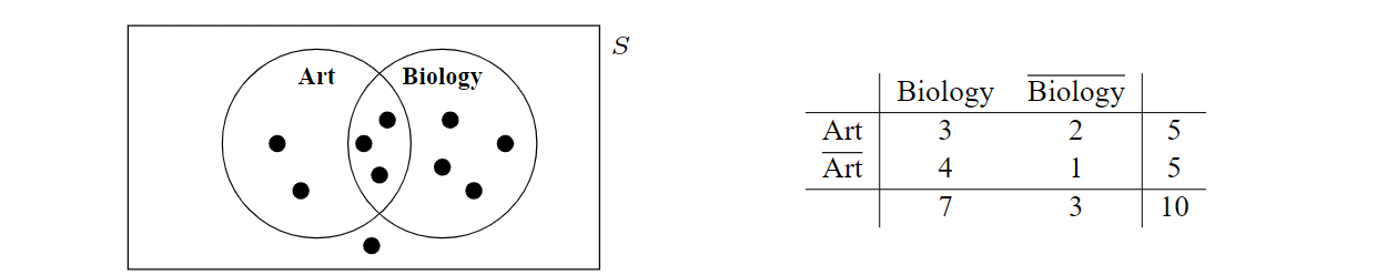
Note that the right hand column shows the total number of pupils that love Biology, and the total that don’t, whilst the final row similarly shows the total number of pupils that love Art, and the total that don’t. These are called marginal totals, and the marginal column and marginal row should both sum to the total number of observations, in this case 17 pupils. The marginal totals can be used to calculate the probability that a randomly chosen pupil loves Art, irrespective of whether they love Biology or not: \(P(\text{Art})=\frac{7}{17}\). If a pupil is randomly chosen and it is first discovered that they love Biology, then the probability they also love Art given that they love Biology is \(\frac{2}{7}\).
This is called a conditional probability and is notated as \(P(\text{Art | Biology})\) or \(P(\text{Art given Biology})\).

The rule for conditional probabilities below is one of the most significant in the context of much of the statistical analysis to come in this course, and it should be carefully learned. Not that, in general, \(\mathbf{P(A|B)\ne P(B|A)}\) and care should be taken not to mix these up.

It should be noted that \(P(\bar{A}|B)=1-P(A|B)\), whilst in general \(P(A|\bar{B})\ne 1-P(A|B)\). Care should be taken to only make use of the valid complement to conditional probabilities.