#> Rows: 4,092
#> Columns: 23
#> $ om <dbl> 192, 27, 38, 57, 60, 61, 50, 52, 96, 108, 113, 117, 119, 76, …
#> $ yr <dbl> 1950, 1950, 1950, 1950, 1950, 1950, 1950, 1950, 1950, 1950, 1…
#> $ mo <dbl> 10, 2, 3, 4, 4, 4, 4, 4, 5, 5, 5, 5, 5, 5, 5, 5, 5, 5, 5, 5, …
#> $ dy <dbl> 1, 27, 27, 28, 28, 28, 2, 3, 11, 16, 22, 24, 29, 4, 4, 4, 7, …
#> $ date <chr> "1950-10-01", "1950-02-27", "1950-03-27", "1950-04-28", "1950…
#> $ time <chr> "21:00:00", "10:20:00", "03:00:00", "14:17:00", "19:05:00", "…
#> $ tz <dbl> 3, 3, 3, 3, 3, 3, 3, 3, 3, 3, 3, 3, 3, 3, 3, 3, 3, 3, 3, 3, 3…
#> $ st <chr> "OK", "OK", "OK", "OK", "OK", "OK", "OK", "OK", "OK", "OK", "…
#> $ stf <dbl> 40, 40, 40, 40, 40, 40, 40, 40, 40, 40, 40, 40, 40, 40, 40, 4…
#> $ stn <dbl> 23, 1, 2, 5, 6, 7, 3, 4, 15, 16, 17, 18, 19, 8, 9, 10, 11, 12…
#> $ mag <dbl> 1, 2, 2, 3, 4, 2, 2, 1, 1, 1, 1, 2, 1, 2, 1, 2, 1, 2, 1, 1, 1…
#> $ inj <dbl> 0, 0, 0, 1, 32, 0, 0, 0, 0, 1, 0, 2, 0, 0, 0, 0, 0, 3, 0, 0, …
#> $ fat <dbl> 0, 0, 0, 1, 5, 0, 0, 0, 0, 0, 0, 0, 0, 0, 0, 0, 0, 0, 0, 0, 0…
#> $ loss <dbl> 4, 4, 3, 5, 5, 4, 4, 3, 2, 3, 0, 4, 2, 4, 3, 5, 0, 4, 3, 4, 3…
#> $ closs <dbl> 0, 0, 0, 0, 0, 0, 0, 0, 0, 0, 0, 0, 0, 0, 0, 0, 0, 0, 0, 0, 0…
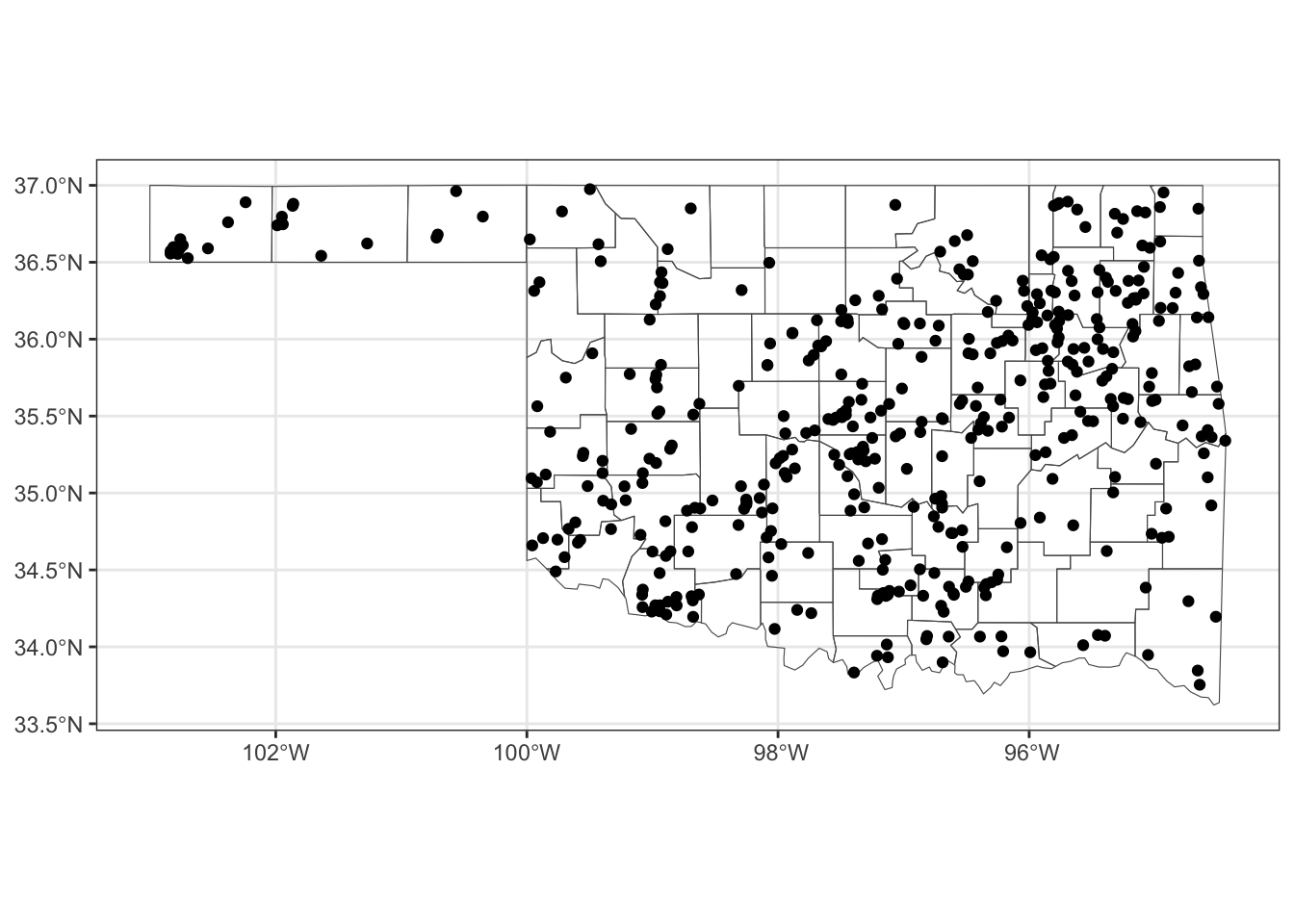
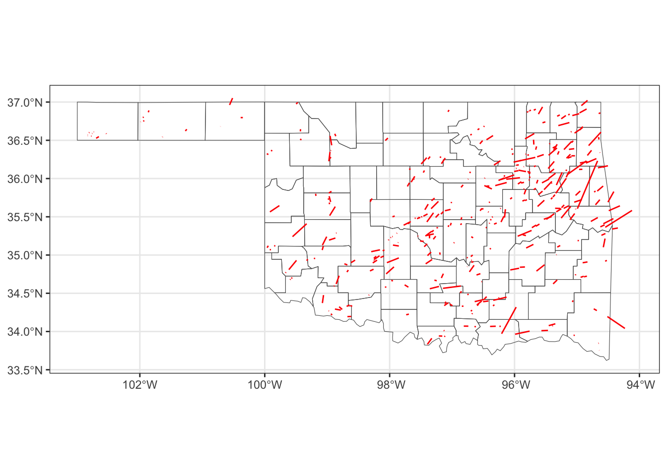
#> $ slat <dbl> 36.73, 35.55, 34.85, 34.88, 35.08, 34.55, 35.82, 36.13, 36.82…
#> $ slon <dbl> -102.52, -97.60, -95.75, -99.28, -96.40, -96.20, -97.02, -95.…
#> $ elat <dbl> 36.8800, 35.5501, 34.8501, 35.1700, 35.1300, 34.5501, 35.8201…
#> $ elon <dbl> -102.3000, -97.5999, -95.7499, -99.2000, -96.3500, -96.1999, …
#> $ len <dbl> 15.8, 2.0, 0.1, 20.8, 4.5, 0.8, 1.0, 1.0, 0.5, 7.3, 1.5, 1.0,…
#> $ wid <dbl> 10, 50, 77, 400, 200, 100, 100, 33, 77, 100, 100, 33, 33, 293…
#> $ fc <dbl> 0, 0, 0, 0, 0, 0, 0, 0, 0, 0, 0, 0, 0, 0, 0, 0, 0, 0, 0, 0, 0…
#> $ geometry <POINT [°]> POINT (-102.52 36.73), POINT (-97.6 35.55), POINT (-95.…