10 Lab 3 Introductory Material
Bring in packages needed for the exercise:
knitr::opts_chunk$set(message = FALSE, warning = FALSE)
# Load required packages
library(sf)
library(raster)
library(terra)
library(gdistance) # Least-cost path analysis package
library(igraph) # Graph theoretical package
library(reticulate)
library(ggplot2)
library(geosphere)
library(sp)
library(dplyr)
10.1 Introduction
For this week’s computer exercise, we will perform least-cost path (LCP) analysis in R using the gdistance package. We will:
- Read and explore a land cover shapefile.
- Rasterize the land cover at different resolutions.
- Create a cost surface and from it build a transition layer.
- Identify connected patches in a raster.
- Calculate and visualize a least-cost path between points.
- Extract path metrics (Euclidean distance, habitat frequency, cost distance).
10.2 Read shapefile and inspect data
Replace with your actual shapefile path and name. This will be the name of the shapefile if you use the 1800 Landcover shapefile. Ensure that ALL the shapefile files are in the same directory (the ones with extensions like .dbf and .prj that contain needed information like the projection of your shapefile and the associated data):
# `st_read()` from the sf package reads a spatial vector file (e.g., shapefile) into an sf object.
LC1800 <- st_read("Land_Cover_Circa_1800.shp")
## Reading layer `Land_Cover_Circa_1800' from data source
## `C:\Users\hanlypat\Desktop\FW840 Spring 2025 Hanly\FW840Hanly\Land_Cover_Circa_1800.shp'
## using driver `ESRI Shapefile'
## Simple feature collection with 151 features and 14 fields
## Geometry type: POLYGON
## Dimension: XY
## Bounding box: xmin: 613547.3 ymin: 239746.1 xmax: 646383.5 ymax: 269168.7
## Projected CRS: NAD83 / Michigan Oblique Mercator## Simple feature collection with 6 features and 14 fields
## Geometry type: POLYGON
## Dimension: XY
## Bounding box: xmin: 633188.9 ymin: 248580 xmax: 646383.5 ymax: 269168.7
## Projected CRS: NAD83 / Michigan Oblique Mercator
## OBJECTID VEGCODE LEGCODE COVERTYPE CNTY_NAME CREATE_UID
## 1 3941 4123 4123 /4124 MIXED OAK FOREST SHIAWASSEE DNRRES_TAYLORG1
## 2 4124 4122 4122 OAK-HICKORY FOREST SHIAWASSEE DNRRES_TAYLORG1
## 3 4222 6227 6226/6227 WET PRAIRIE SHIAWASSEE DNRRES_TAYLORG1
## 4 4242 4122 4122 OAK-HICKORY FOREST SHIAWASSEE DNRRES_TAYLORG1
## 5 4246 4122 4122 OAK-HICKORY FOREST SHIAWASSEE DNRRES_TAYLORG1
## 6 4250 6227 6226/6227 WET PRAIRIE SHIAWASSEE DNRRES_TAYLORG1
## CREATE_DTS UPDATE_UID UPDATE_DTS GENERALIZE SHAPE_STAr SHAPE_STLe
## 1 2001-10-16 DNRRES\\TAYLORG1 2002-03-04 41 126808463.3 368825.771
## 2 2001-10-16 DNRRES\\TAYLORG1 2002-03-04 41 52295096.2 150099.336
## 3 2001-10-16 DNRRES\\TAYLORG1 2002-03-05 6 2739126.2 27967.043
## 4 2001-10-16 DNRRES\\TAYLORG1 2002-03-04 41 1059031.7 5668.901
## 5 2001-10-16 DNRRES\\TAYLORG1 2002-03-04 41 6770350.8 30818.334
## 6 2001-10-16 DNRRES\\TAYLORG1 2002-03-05 6 186305.9 2509.120
## ShapeSTAre ShapeSTLen geometry
## 1 126808462.0 368825.771 POLYGON ((633258.5 268480.5...
## 2 52295096.3 150099.336 POLYGON ((640436.1 258635.3...
## 3 2739126.1 27967.043 POLYGON ((633909.4 254491.4...
## 4 1059031.7 5668.901 POLYGON ((633590.6 253850.1...
## 5 6770350.7 30818.334 POLYGON ((634393.8 253394, ...
## 6 186305.9 2509.120 POLYGON ((637573.1 253888, ...10.3 Classify and visualize patches
Inspect and determine what the patches and mosaic will be for your landscape. Here, I am setting LAKE/RIVER to patches and everything else to mosaic. You can also lump multiple types into patches as well (e.g., multiple types of forest).
# Classify Lakes/Rivers as "Patch", everything else as "Mosaic"
LC1800$type <- ifelse(LC1800$COVERTYPE == "LAKE/RIVER", "Patch", "Mosaic")

# Plot the original land cover categories
ggplot() +
  geom_sf(data = LC1800, aes(fill = COVERTYPE), color = "gray20", size = 0.1) +
  theme_minimal() +
  theme(legend.position = "right",
        legend.title = element_text(size = 12, face = "bold"),
        legend.text = element_text(size = 10),
        panel.grid = element_blank(),
        axis.text = element_blank(),
        axis.ticks = element_blank()) +
  labs(title = "1800 Land Cover Map")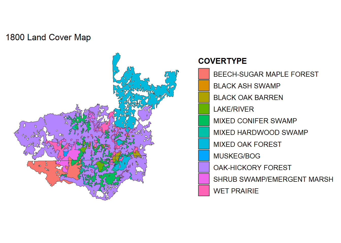
# Plot the new Patch/Mosaic classification
ggplot() +
  geom_sf(data = LC1800, aes(fill = type), color = "gray20", size = 0.1) +
  theme_minimal() +
  theme(legend.position = "right",
        legend.title = element_text(size = 12, face = "bold"),
        legend.text = element_text(size = 10),
        panel.grid = element_blank(),
        axis.text = element_blank(),
        axis.ticks = element_blank()) +
  labs(title = "1800 Patch/Mosaic Map")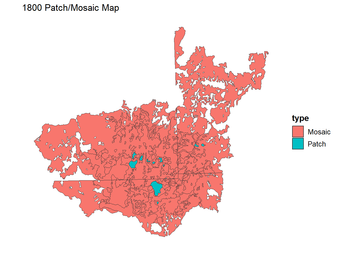
10.4 Rasterize our shapefile
To use our landcover (or other shapefile) data in gdistance, we must first convert our shapefile to a raster. This conversion is useful for many analyses since many packages are designed only for raster format data, and the procedures may only make sense for gridded data. One of the decision points is the resolution of the raster you generate from the shapefile. Here, I rasterize the polygon data at the 10m, 100m, and 1000m pixel resolutions to explore the grain size created.
raster() from the ‘raster’ package creates an empty raster layer with a specified resolution and extent.
rasterize() burns the polygon data into the raster, assigning values (here, VEGCODE) to overlapping cells.
Note: This may take awhile if your shapefiles are very complex or very large.
# Ensure VEGCODE is numeric for rasterization
LC1800$VEGCODE <- as.numeric(LC1800$VEGCODE)

# Determine the bounding extent of LC1800
extent1800 <- extent(LC1800)

# Create empty rasters at different resolutions
r10   <- raster(extent1800,  res = 10,   crs = st_crs(LC1800)$proj4string)
r100  <- raster(extent1800,  res = 100,  crs = st_crs(LC1800)$proj4string)
r1000 <- raster(extent1800,  res = 1000, crs = st_crs(LC1800)$proj4string)

# Rasterize using "VEGCODE" as the attribute field
raster_10m   <- rasterize(LC1800, r10,   field = "VEGCODE")
raster_100m  <- rasterize(LC1800, r100,  field = "VEGCODE")
raster_1000m <- rasterize(LC1800, r1000, field = "VEGCODE")

# Compare them side by side
par(mfrow = c(1,3))
plot(raster_10m,   main = "Land Cover (10m)",   col = terrain.colors(10))
plot(raster_100m,  main = "Land Cover (100m)",  col = terrain.colors(10))
plot(raster_1000m, main = "Land Cover (1000m)", col = terrain.colors(10))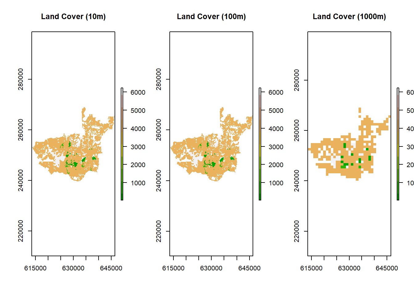
10.5 Identify the patch class and mask
For my example, I am focusing on LAKE/RIVER (VEGCODE 52). Note that these codes are specific to your raster and data. We can isolate these cells in the 100m raster, creating a binary yes/no for patches:
# Print a reference table of VEGCODE -> COVERTYPE
print(LC1800[!duplicated(LC1800$VEGCODE), c('VEGCODE','COVERTYPE')], n = 30)
## Simple feature collection with 14 features and 2 fields
## Geometry type: POLYGON
## Dimension: XY
## Bounding box: xmin: 616176.7 ymin: 242479.2 xmax: 646383.5 ymax: 269168.7
## Projected CRS: NAD83 / Michigan Oblique Mercator
## VEGCODE COVERTYPE geometry
## 1 4123 MIXED OAK FOREST POLYGON ((633258.5 268480.5...
## 2 4122 OAK-HICKORY FOREST POLYGON ((640436.1 258635.3...
## 3 6227 WET PRAIRIE POLYGON ((633909.4 254491.4...
## 9 4233 MIXED CONIFER SWAMP POLYGON ((635275.7 253234.5...
## 12 52 LAKE/RIVER POLYGON ((636042.3 252592.9...
## 14 6221 SHRUB SWAMP/EMERGENT MARSH POLYGON ((637322.9 252620.1...
## 28 4141 BLACK ASH SWAMP POLYGON ((633690.9 250006.1...
## 31 332 BLACK OAK BARREN POLYGON ((637202 249439.8, ...
## 58 41 MIXED HARDWOOD SWAMP POLYGON ((630071.4 246846.3...
## 60 4121 BEECH-SUGAR MAPLE FOREST POLYGON ((626703.5 247734.1...
## 66 414 MIXED HARDWOOD SWAMP POLYGON ((635696.1 247057, ...
## 71 6123 SHRUB SWAMP/EMERGENT MARSH POLYGON ((636600.7 246603.7...
## 86 42 MIXED CONIFER SWAMP POLYGON ((632618.2 244551.6...
## 137 6121 MUSKEG/BOG POLYGON ((624229.5 249496.7...# I am printing the top 30 lines in the previous code, you may need more if you have more or less.
# Create a mask to isolate LAKE/RIVER (VEGCODE = 52)
lake_river_mask <- raster_100m
lake_river_mask[lake_river_mask != 52] <- NA # Set non-lake/river to NA
lake_river_mask[lake_river_mask == 52] <- 1 # Set lake/river to 1
# Plot the lake/river mask
plot(lake_river_mask, main = "Target Patches: LAKE/RIVER", col = "blue")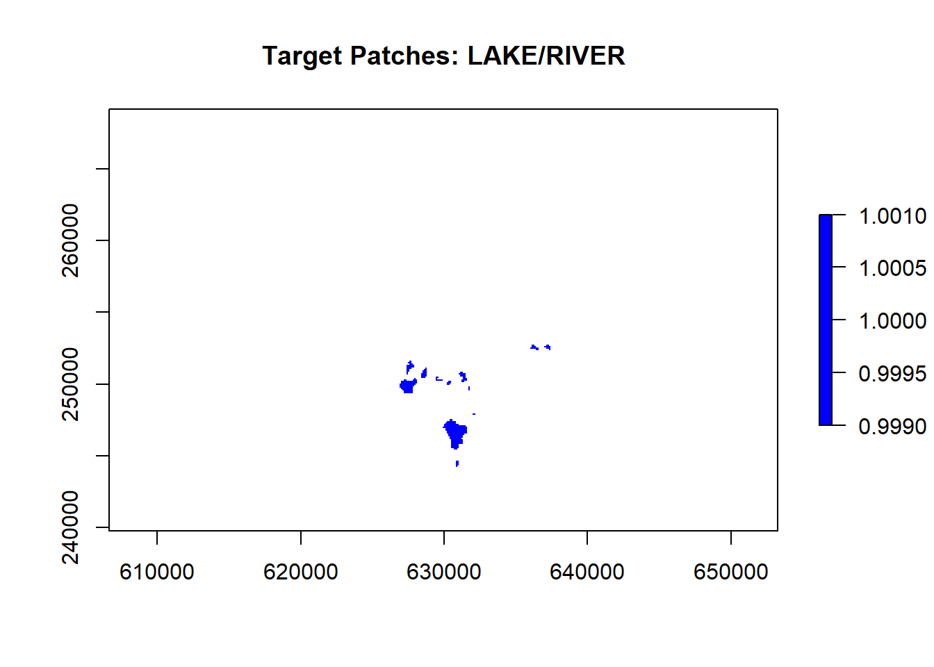
10.6 Constructing a cost-surface
A cost surface is a raster where each cell’s value indicates the cost (or difficulty) of traversing that cell. We define cost values for each VEGCODE. Here I am showing how to specify each cost for each VEGCODE using a manual classification.
reclassify() from raster updates values based on a table or matrix.
By assigning larger numbers, we indicate more difficulty for that land cover type.
# Take our 100m raster as a base
cost_surface <- raster_100m

# Define specific cost values for each VEGCODE
costs <- data.frame(
  VEGCODE = c(41, 42, 52, 332, 414, 4121, 4122, 4123, 4141, 4233, 6121, 6123, 6221, 6227),
  cost    = c(2,  1,  1.5, 3,   5.6, 8.2,  9,    8,    5.5,  5.6,  5.1,   5.3,   6.1,  6)
)

# Reclassify the cost surface according to the table
cost_surface_reclassified <- reclassify(cost_surface, costs)

# Replace NA with a higher cost (10) to avoid ignoring them
cost_surface_reclassified[is.na(cost_surface_reclassified)] <- 10

# Plot the final cost surface
plot(cost_surface_reclassified, main = "Cost Surface", col = terrain.colors(100))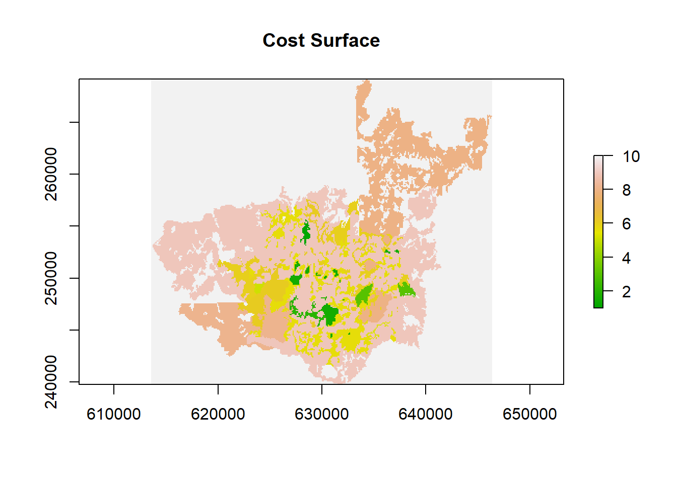
10.7 Building a transition layer
In gdistance, we need a transition layer that dictates how movement occurs from one cell to its neighbor. This transition layer is derived from the cost surface. Today, we will use a simple transition function but there are more complex ones or ones more suitable for elevational change or other specific processes:
The transitionFunction = function(x) 1/mean(x) sets up how to compute the “cost” or “conductance” between adjacent cells. Inverse cost implies that higher cost = lower conductance.
directions = 4 restricts adjacency to up, down, left, and right.
geoCorrection() adjusts distances if the data is in a geographic CRS.
# Create a transition object
surf <- transition(
  x = cost_surface_reclassified,
  transitionFunction = function(x) 1 / mean(x), # Set the transition function, here
  directions = 4
)

# Geo-correct if working in geographic coordinates
surf <- geoCorrection(surf, type = "c")

# Convert to raster for visualization
plot(raster(surf), main = "Transition Object Layer")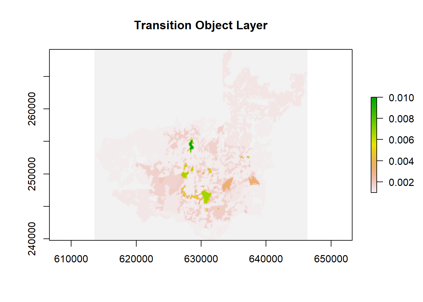
10.8 Identify and count patches
We can look for patches (connected areas) where VEGCODE == 42, our lakes/rivers, by creating a binary raster and then using clump().
# Identify pixels where VEGCODE == 42
patch <- raster_100m == 42

# Replace NA with 0
patch[is.na(patch)] <- 0

# Identify connected patches (4-direction connectivity)
patches <- clump(patch, directions = 4)

# Count how many distinct patches exist
num_patches <- max(values(patches), na.rm = TRUE)
print(paste("Number of lake/river patches:", num_patches))
## [1] "Number of lake/river patches: 5"10.9 Extract patch coordinates
Once we have our raster with binary patches, we can convert it to polygons and compute centroids for each patch. Alternatively, we could have done this with the original shapefile, but we may have lost some of the original patches depending on the resolution we set for rasterization.
rasterToPolygons() groups the cells of each patch into a polygon, labeled by the patch ID.
coordinates() yields the polygon centroids as an (x,y) matrix.
# Convert patches raster to polygons
patches_poly <- rasterToPolygons(patches, dissolve = TRUE)

# Compute centroids for each polygon
centroids <- coordinates(patches_poly)

# Convert to a data frame
centroid_df <- data.frame(
  patch_id = patches_poly$clumps,
  lon = centroids[,1],
  lat = centroids[,2]
)

# Inspect the results
print(centroid_df)
## patch_id lon lat
## 1 1 628430.6 255552.1
## 2 2 628437.9 254411.8
## 3 3 627922.3 253643.7
## 4 4 628397.3 253218.7
## 5 5 632563.9 244652.110.10 Calculate a least-cost path
We are FINALLY ready to calculate our least-path now that we have our transition layer and our patch coordinates. Using the transition layer, we compute a least-cost path between two selected patch centroids:
shortestPath() finds the route that minimizes total cost between the start and end points, returning a SpatialLines object. There is no randomness occurring here, and is based purely on the values we provide in the transition layer.
# Example start and end points from our centroid table
start <- cbind(centroid_df$lon[1], centroid_df$lat[1])
end   <- cbind(centroid_df$lon[5], centroid_df$lat[5])

# Compute the shortest path
cost_path <- gdistance::shortestPath(surf, start, end, output = "SpatialLines")

# Plot the path
plot(raster(surf), main = "Least-Cost Path", col = terrain.colors(100), legend = TRUE)
lines(cost_path, col = "purple", lwd = 2)

# Add start (blue) and end (red) points
points(start[1], start[2], col = "blue", pch = 16, cex = 2)
points(end[1], end[2], col = "red", pch = 16, cex = 2)

text(start[1], start[2], labels = "Start", pos = 3, col = "blue", font = 2)
text(end[1], end[2], labels = "End", pos = 3, col = "red", font = 2)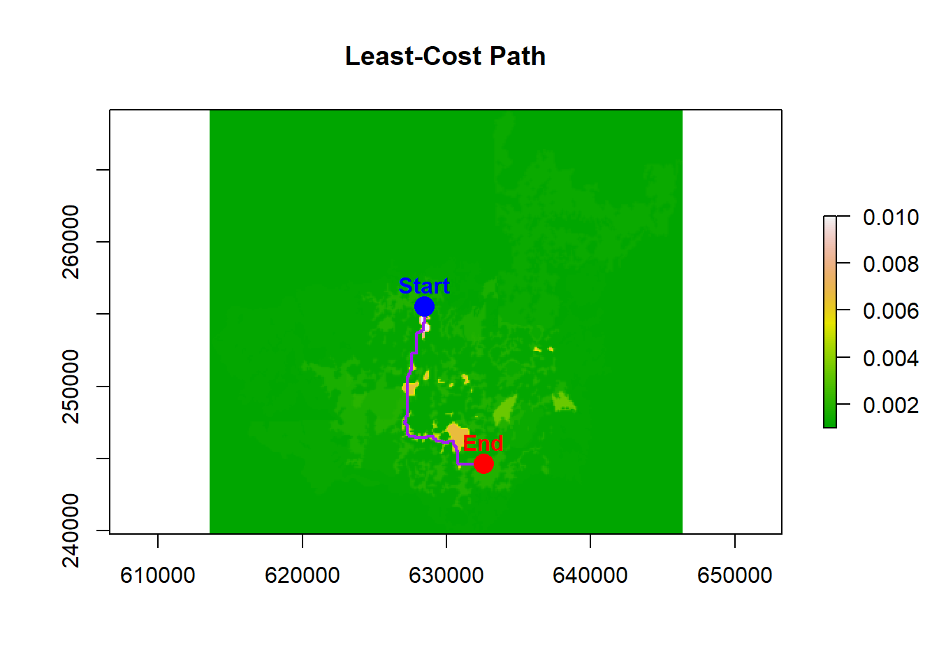
10.11 Example path metrics
We can explore different metrics describing our route or for the study extent. I just have a few here that are easy to compute, many require additional computation to add randomness, error, or comparison to random paths.
- Euclidean distance between our start and end points:
## [1] 11657.38- Habitat frequency along path, counting the types of cells encountered during the least-cost travel:
# Extract the raster values along the path
path_habitats <- extract(raster_100m, cost_path)
table(path_habitats) / length(path_habitats)
## path_habitats
## 41 42 52 4122 4233
## 55 30 36 31 34- Multi-point path cost distances can be calculated by giving the
costDistance()function more than two sets of coordinates. It will calculate the pair-wise path costs for all points given. So, if you have huge number of points this could take a long time:
# Compute pairwise cost distances among all patch centroids
cost_dist <- costDistance(surf, cbind(centroid_df$lon, centroid_df$lat))
cost_dist
## 1 2 3 4
## 2 2300
## 3 4400 2100
## 4 4300 2000 2900
## 5 66240 63940 61840 62670