6.22 Ordinal logistic regression
An ordinal variable is a categorical variable in which the levels have a natural ordering (e.g., depression categorized as Minimal, Mild, Moderate, Moderately Severe, and Severe). Ordinal logistic regression can be used to assess the association between predictors and an ordinal outcome. You can fit an ordinal logistic regression model in R with MASS::polr() (proportional odds logistic regression) (Ripley 2023).
WARNING: Use the syntax MASS::polr() rather than loading the MASS library, as loading it masks the select() function in both gtsummary() and tidyverse() leading to errors when using those packages.
NOTE: The proportional odds model is only one possible model for ordinal data. See Greenland (1994) for a discussion of an alternative model which may be a better choice if, for example, the underlying distribution is truly ordinal (as opposed to having an ordinal variable that is the result of collapsing an underlying continuous variable into groups), or the proportional odds assumption is not met.
6.22.1 Ordinal model
In binary logistic regression, the outcome \(Y\) has two levels. If the two levels are referred to as 0 and 1, we model the probability that \(Y = 1\). What if you have an outcome with more than two levels, and the levels are ordered? The ordinal logistic regression model, as parameterized by MASS::polr(), for an outcome \(Y\) with levels \(\ell = 1, 2, ..., L\) is
\[\begin{equation} \ln{\left( \frac{P(Y \leq \ell)}{P(Y > \ell)} \right)} = \zeta_{\ell} - \eta_1 X_1 - \eta_2 X_2 - \ldots - \eta_K X_K \tag{6.3} \end{equation}\]
for each level \(\ell = 1, 2, ..., L-1\). Equation (6.3) only works for levels up to \(L-1\) because if we went up to \(L\) we would have \(P(Y > L) = 0\) in the denominator. The letter \(\zeta\) is pronounced “zeta” and the letter \(\eta\) is pronounced “eta”. Just like binary logistic regression, the left-hand side is the log-odds of a probability, but now instead of a probability of an outcome being at one level, it is the cumulative probability of an outcome being at any level up to and including a specified level.
How do we interpret the regression terms?
- \(\zeta_{\ell}\) is an intercept and represents the log-odds of \(Y \leq \ell\) when all the predictors are at 0 or their reference level. Thus, \(P(Y \leq \ell)\) is the inverse-logit of \(\zeta_{\ell}\). Unlike other forms of regression we have worked with, an ordinal logistic regression model has multiple intercepts, one for each level of \(Y\) from \(1\) to \(L-1\).
- Each \(-\eta_k\) for \(k = 1, 2, ..., K\) is the log of the odds ratio comparing the odds of \(Y \leq \ell\) between individuals who differ by 1-unit in \(X_k\) (or comparing individuals at a level of \(X_k\) and the reference level).
- \(e^{-\eta_k}\) is the odds ratio comparing the odds of \(Y \leq \ell\) between those differing by 1-unit in \(X_k\).
- \(e^{\eta_k}\) is the odds ratio comparing the odds of \(Y > \ell\) between those differing by 1-unit in \(X_k\).
Since MASS::polr() returns estimates of \(\eta\), not \(-\eta\), an OR > 1 corresponds to greater odds of the outcome being at higher levels.
For each individual level \(\ell\), this is similar to a binary logistic regression for a dichotomized version of \(Y\) where the two levels are \(Y > \ell\) and \(Y \leq \ell\). However, the ordinal logistic regression model goes further. It fits the model for all the levels of \(Y\) at the same time, estimates an intercept for each level of the outcome (other than the highest level), and assumes the regression coefficient for each predictor \(X_k\) is the same for all \(\ell\). This assumption is called the proportional odds assumption, because it implies that the odds ratio for a predictor \(X\) is the same at all levels of \(Y\) – no matter where you split \(Y\) into \(Y > \ell\) and \(Y \leq \ell\), the resulting odds at any two values of \(X\) are proportional (have the same ratio).
6.22.2 Transforming a continuous outcome into an ordinal outcome
In addition to outcomes that are inherently ordinal, we often encounter outcomes that are continuous, highly skewed, and bounded below by 0. When fitting a linear regression to such an outcome, the regression assumptions can fail and no transformation is effective at resolving the issues. One solution is to collapse the outcome into an ordinal outcome.
NOTE: This section is necessary for Example 6.5, but if you are referring to this chapter in order to carry out an analysis of an outcome that is already coded as ordinal, skip ahead to Section 6.22.3.
Example 6.5: The PHQ-9 is the depression module of the Patient Health Questionnaire (Kroenke, Spitzer, and Williams 2001; Kroenke and Spitzer 2002). It consists of nine questions, each scored from 0 to three and summed for a total score ranging from 0 to 27. Scores in the ranges 0-4, 5-9, 10-14, 15-19, and 20-27 are labeled as Minimal, Mild, Moderate, Moderately Severe, and Severe depression, respectively. A summary and histogram of PHQ-9 scores (phq9) from the NHANES examination teaching dataset (nhanes1718_adult_exam_sub_rmph.Rdata) reveals that it has many zeros and is highly skewed. Create a three-level ordinal variable corresponding to Minimal, Mild, and Moderate to Severe depression.
## [1] 278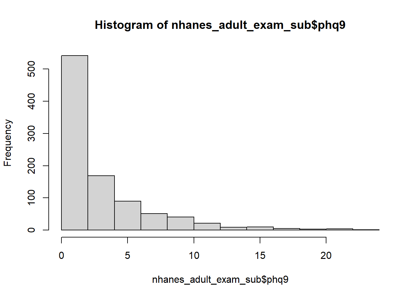
We demonstrate here two methods for turning the raw PHQ-9 variable, which ranges from 0 to 27, into a three-level variable. The cut() function is very useful but a little tricky to get right due to the way it requires you to specify whether intervals are closed on the left and/or right. A nice feature of cut() is that the result is formatted as a factor with levels labeled with the interval definitions. After trying out the different combinations of right and include.lowest, we find we need right = F and include.lowest = T to get the intervals we want.
# Options for cut()
# right = T leads to intervals closed on the right
# right = F leads to intervals open on the right (unless include.lowest=T)
# For right = T, include.lowest = T leads to the FIRST interval closed on the left
# For right = F, include.lowest = T leads to the LAST interval closed on the right
# (so for right = F, "include.lowest" is better thought of as "include.highest")
# right include.lowest  first_interval  middle_intervals last_interval
# T     T               [0,5]           (5, 10]          (10, 27]
# T     F               (0,5]           (5, 10]          (10, 27]
# F     T               [0,5)           [5, 10)          [10, 27]
# F     F               [0,5)           [5, 10)          [10, 27)

# Create three-level PHQ-9 total using cut
nhanes <- nhanes_adult_exam_sub %>%
  mutate(depression = cut(phq9,
                          c(0, 5, 10, 27),
                          right = F,
                          include.lowest = T))

# Is it a factor?
is.factor(nhanes$depression)
## [1] TRUE# Did all values go to the right category, and no new NAs?
table(nhanes_adult_exam_sub$phq9, nhanes$depression, useNA = "ifany")##
## [0,5) [5,10) [10,27] <NA>
## 0 278 0 0 0
## 1 153 0 0 0
## 2 110 0 0 0
## 3 86 0 0 0
## 4 83 0 0 0
## 5 0 57 0 0
## 6 0 33 0 0
## 7 0 27 0 0
## 8 0 24 0 0
## 9 0 21 0 0
## 10 0 0 20 0
## 11 0 0 14 0
## 12 0 0 7 0
## 13 0 0 4 0
## 14 0 0 5 0
## 15 0 0 7 0
## 16 0 0 3 0
## 18 0 0 5 0
## 19 0 0 1 0
## 20 0 0 2 0
## 21 0 0 3 0
## 22 0 0 1 0
## 24 0 0 1 0
## <NA> 0 0 0 55# Check the range of values in each category
tapply(nhanes_adult_exam_sub$phq9, nhanes$depression, range)## $`[0,5)`
## [1] 0 4
##
## $`[5,10)`
## [1] 5 9
##
## $`[10,27]`
## [1] 10 24##
## [0,5) [5,10) [10,27] <NA>
## 710 162 73 55The derivation was correct, although in this dataset the maximum value was 24 rather than the maximum possible of 27.
Another approach is to use case_when() in which we specify a series of logical statements to define the intervals, and then convert the result to a factor. The new variable takes on the value 1 (the value after the ~ in the first row) if the first condition is met, the value 2 if the first condition is not met but the second is, and so on. This leads to the exact same result as cut(). Regardless of which you use, always check the derivation afterward to make sure your new variable is as intended.
# Create three-level PHQ-9 total using case_when
nhanes <- nhanes_adult_exam_sub %>%
mutate(depression = case_when(phq9 < 5 ~ 1,
phq9 < 10 ~ 2,
phq9 >= 10 ~ 3),
depression = factor(depression,
levels = 1:3,
labels = c("Minimal",
"Mild",
"Moderate to Severe")))# Check derivation (results identical to before)
# Is it a factor?
is.factor(nhanes$depression)
# Did all values go to the right category, and no new NAs?
table(nhanes_adult_exam_sub$phq9, nhanes$depression, useNA = "ifany")
# Check the range of values in each category
tapply(nhanes_adult_exam_sub$phq9, nhanes$depression, range)
##
## Minimal Mild Moderate to Severe <NA>
## 710 162 73 556.22.3 Make sure you know what probabilities polr() is modeling
Before fitting an ordinal logistic regression, check the ordering of the outcome variable. An OR > 1 corresponds to a risk factor that is associated with greater probability of higher levels of the outcome variable. Therefore, typically, the ordering desired for an outcome variable is from less severe to more severe. Whatever the ordering desired, check using levels() and, if needed, reorder using factor().
Example 6.5 (continued): What is the ordering for the outcome depression? Is that the ordering desired?
## [1] "Minimal" "Mild" "Moderate to Severe"The ordering is from less severe to more severe. We would like an OR > 1 to correspond to a risk factor associated with greater probability of a more severe outcome, so this is the ordering desired.
The code below demonstrates how to reorder the levels of an outcome variable, if needed. For this demonstration, we create an artificial dataset with a factor x that is ordered from high to low severity (the opposite of what we would like).
# Just for this example (skip if not needed)
set.seed(5)
dat <- data.frame(x = factor(sample(1:3, 100, replace=T),
                             levels = 1:3,
                             labels = c("High", "Med", "Low")))

# Current level ordering
levels(dat$x)
## [1] "High" "Med" "Low"Currently, the levels are in order from high to low. Let’s reverse that ordering.
# Reorder
dat <- dat %>%
  mutate(x_new = factor(x,
                        levels = c("Low", "Med", "High")))

# Check derivation
table(dat$x, dat$x_new, useNA = "ifany")
##
## Low Med High
## High 0 0 34
## Med 0 32 0
## Low 34 0 0## [1] "Low" "Med" "High"The new variable x_new is exactly the same as the old variable x (see the two-way “Check derivation” table) except that now the levels are ordered from low to high.
6.22.4 Separation
As with binary logistic regression, an ordinal logistic regression model could suffer from separation if there are levels of a categorical predictor at which the outcome can be perfectly predicted. But, since an ordinal model works with cumulative probabilities, there are some situations when a zero in the two-way table of a categorical predictor vs. the ordinal outcome does not cause a problem. In particular, if there is a zero in just one cell then the model may still fit and provide reasonable results. For example, consider the following two-way table of a Yes/No predictor vs. a three-level ordinal outcome.
No individuals with “No” for the predictor were at level 2 of the outcome. However, despite this zero, an ordinal logistic regression model will converge and produce reasonable results. If the single zero is in the first or last level of the outcome, however, the model may converge but violate the proportional odds assumption (see Section 6.22.10) because there will be separation in one of the binary logistic regressions used to check the assumption.
Being able to perfectly predict an ordinal outcome at a level of a predictor requires zeros in the table at all but one level of the outcome, such as the following two-way table.
An ordinal logistic regression fit to the data from the above table will suffer from quasi-complete separation. In this particular example, the model seems to converge but produces a huge odds ratio and an error when attempting to compute confidence intervals.
To diagnose separation for an ordinal logistic regression, fit the model and examine the output for errors, warnings, and nonsense output (large standard errors, inverse logit of intercepts near 0 or 1, or odds ratios approaching 0 or infinite). If there seems to be an issue, check for zeros using two-way tables of categorical predictors vs. the outcome to determine which predictor is the problem, or if the problem is a sparse outcome. If the problem is a predictor, then filter, collapse, or remove the predictor (see Section 6.10.4). If the problem is the outcome, then filter or collapse the outcome. If doing so results in a two-level outcome, then the model is reduced to a binary logistic regression.
6.22.5 Fitting the model
This section demonstrates how to use MASS::polr() to fit the ordinal logistic regression model. Include the Hess=T option to speed up subsequent calls to summary().
Example 6.5 (continued): Use ordinal logistic regression to test the association between depression (depression) and engaging in vigorous recreational activities (Yes/No, PAQ650).
## Call:
## MASS::polr(formula = depression ~ PAQ650, data = nhanes, Hess = T)
##
## Coefficients:
##          Value Std. Error t value
## PAQ650No 0.347      0.173       2
##
## Intercepts:
##                         Value  Std. Error t value
## Minimal|Mild             1.360  0.151      9.037
## Mild|Moderate to Severe  2.739  0.180     15.220
##
## Residual Deviance: 1347.12
## AIC: 1353.12
## (55 observations deleted due to missingness)
The output does not include any p-values; we will compute them in Section 6.22.8.
6.22.6 Interpreting the coefficients
Intercepts
Since the outcome in our example has three levels, there are two intercepts, stored in a component of the model object called zeta. These are log-odds of cumulative probabilities, which can be seen by using ilogit() (in Functions_rmph.R) and comparing the result to the raw cumulative probabilities at the reference level of the predictor (PAQ650 = “Yes”).
##            Minimal|Mild Mild|Moderate to Severe
## 0.7958 0.9393## Minimal Mild Moderate to Severe
## 0.7963 0.9370 1.0000In other words, for the predictor at its reference level, the inverse logit of the first intercept is \(P(Y \leq 1)\) and the inverse logit of the second intercept is \(P(Y \leq 2)\). There is no third intercept because \(Y\) only has three levels, so \(P(Y \leq 3)\) is always 1 and there is no need to estimate it.
The first intercept is the log odds of Minimal depression. The label “Minimal|Mild” is expressing the fact that the odds correspond to \(P(\textrm{Depression} \leq \textrm{Minimal}) / P(\textrm{Depression} > \textrm{Minimal})\) which is equivalent to \(P(\textrm{Depression} \leq \textrm{Minimal}) / P(\textrm{Depression} \geq \textrm{Mild})\), hence the label “Minimal|Mild”. Similarly, the second intercept is the log odds of “up to Mild depression” (which includes Minimal and Mild). The label “Mild|Moderate to Severe” is expressing the fact that the odds correspond to \(P(\textrm{Depression} \leq \textrm{Mild}) / P(\textrm{Depression} \geq \textrm{Moderate to Severe})\).
Conclusion: The estimated proportion of individuals with Minimal depression is 0.796 and the estimated proportion of individuals with Minimal or Mild depression is 0.939.
NOTE: Above, the estimated cumulative probabilities are similar but not exactly equal to the corresponding raw cumulative probabilities. Had there been no predictor in the model, these would be identical, as shown below.
##            Minimal|Mild Mild|Moderate to Severe
## 0.7513 0.9228## Minimal Mild Moderate to Severe
## 0.7513 0.9228 1.0000Predictor coefficients
Each predictor’s coefficient is the log odds ratio for that predictor. Exponentiate to get OR = \(e^\eta\) and use confint() and exponentiate to compute a 95% confidence interval for the OR.
# OR and 95% CI
CI <-  confint(fit.olr)
data.frame(
  OR    = exp(fit.olr$coefficients),
  lower = exp(CI[1]),
  upper = exp(CI[2])
)
## OR lower upper
## PAQ650No 1.415 1.013 2.001# Use the following if there is more than one predictor row
# e.g., CI[,1] instead of CI[1] since CI is now a matrix
data.frame(
OR = exp(fit.olr$coefficients),
lower = exp(CI[,1]),
upper = exp(CI[,2])
)Conclusion: Individuals who do not engage in vigorous recreational activities have 41.5% greater odds of more severe depression (OR = 1.415, 95% CI = 1.013, 2.001).
NOTE: The interpretation of the OR > 1 for vigorous recreational activity is expressed as corresponding to “greater odds of more severe depression” because the probability is shifting toward higher values of the outcome (illustrated in the next section). In a binary logistic regression of the outcome “depression” (yes vs. no), we would just say “greater odds of depression”.
6.22.7 What does an OR > 1 mean?
In the end, practically, an ordinal logistic regression results in exactly the same number of ORs as a binary logistic regression – one for each continuous predictor and one less than the number of levels for each categorical predictor. When interpreting the effect of a predictor on the outcome, the interpretation will be very similar between binary and ordinal logistic regression.
For example, if you fit a binary logistic regression and estimate the OR for a continuous variable \(X\) to be 1.50, you conclude that those with 1-unit greater \(X\) have 50% greater odds of the outcome. Implied in this statement is that they have 50% greater odds of having \(Y = 1\) compared to \(Y = 0\) because the odds are the ratio \(P(Y = 1) / P(Y = 0)\). The interpretation of an OR of 1.50 in an ordinal logistic regression is that those with a 1-unit greater \(X\) have 50% greater odds of having a greater outcome – 50% greater odds of \(Y > 1\) compared to \(Y \leq 1\), 50% greater odds of \(Y > 2\) compared to \(Y \leq 2\), …, and 50% greater odds of \(Y > L-1\) compared to \(Y \leq L-1\).
Again, in an ordinal logistic regression, an OR > 1 means that one level of a predictor is associated with greater probability of more severe levels of the outcome. This section goes a bit deeper to illustrate what that statement means, as well as how the aforementioned proportional odds assumption constrains the shift in probability toward more severe levels.
Example 6.5 (continued): To further clarify the interpretation of an OR estimated from an ordinal model, consider the distribution of depression at each level of vigorous recreational activity. The fact that the OR is larger than 1 corresponds to the probability distribution shifting to more severe levels of depression when moving from the reference level to the non-reference level.
TAB.Yes <- table(nhanes$depression[nhanes$PAQ650 == "Yes"])
TAB.No  <- table(nhanes$depression[nhanes$PAQ650 == "No"])

OUT <- rbind(prop.table(TAB.Yes),
             prop.table(TAB.No))
rownames(OUT) <- c("P(Depression) @ Physical activity = Yes (ref)",
                   "P(Depression) @ Physical activity = No")

round(OUT,        3)
## Minimal Mild Moderate to Severe
## P(Depression) @ Physical activity = Yes (ref) 0.796 0.141 0.063
## P(Depression) @ Physical activity = No 0.733 0.184 0.083Individuals in the non-reference level (in the second row of the table above) have a greater chance of having more severe depression. This “shift toward higher probabilities” happens in a manner that is constrained by the proportional odds assumption. To help clarify this assumption, consider the following set of empirical ORs (based on the raw data, not estimated from a model), each comparing the odds of being in higher levels vs. lower levels at different outcome cutoff values.
# Empirical ORs, computed based on raw probabilities

# Odds of > Minimal vs. <= Minimal at PA = Yes
ODDS.Y <- (0.141 + 0.063) / (1 - 0.141 - 0.063)

# Odds of > Minimal vs. <= Minimal at PA = No
ODDS.N <- (0.184 + 0.083) / (1 - 0.184 - 0.083)

OR1.RAW <- ODDS.N / ODDS.Y

# Odds of > Mild vs. <= Mild at PA = Yes
ODDS.Y <- 0.063 / (1 - 0.063)

# Odds of > Mild vs. <= Mild at PA = No
ODDS.N <- 0.083 / (1 - 0.083)

OR2.RAW <- ODDS.N / ODDS.Y

c(OR1.RAW, OR2.RAW)
## [1] 1.421 1.346Next, consider the corresponding ORs computed using probabilities estimated from the model, and compare them to the empirical ORs above, as well as to the OR computed by exponentiating the estimated regression coefficient from the model. This code introduces the use of predict() with a polr object, a topic which will be discussed in Section 6.22.9.
# Distributions estimated from the model
predict(fit.olr,
        data.frame(PAQ650 = c("Yes", "No")),
        type="p")
## Minimal Mild Moderate to Severe
## 1 0.7958 0.1435 0.06073
## 2 0.7336 0.1826 0.08384# ORs computed from probabilities estimated by the model
# Odds of > Minimal vs. <= Minimal at PA = Yes
ODDS.Y <- (0.1434646 + 0.06072555) / (1 - 0.1434646 - 0.06072555)
# Odds of > Minimal vs. <= Minimal at PA = No
ODDS.N <- (0.1825769 + 0.08383594) / (1 - 0.1825769 - 0.08383594)
OR1.EST <- ODDS.N / ODDS.Y
# Odds of > Mild vs. <= Mild at PA = Yes
ODDS.Y <- 0.06072555 / (1 - 0.06072555)
# Odds of > Mild vs. <= Mild at PA = No
ODDS.N <- 0.08383594 / (1 - 0.08383594)
OR2.EST <- ODDS.N / ODDS.Y
list("Empirical ORs" = c(OR1.RAW, OR2.RAW),
"ORs computed from estimated probabilities" = c(OR1.EST, OR2.EST),
"OR = exp(beta) from model" = exp(fit.olr$coefficients["PAQ650No"]))## $`Empirical ORs`
## [1] 1.421 1.346
##
## $`ORs computed from estimated probabilities`
## [1] 1.415 1.415
##
## $`OR = exp(beta) from model`
## PAQ650No
## 1.415This illustrates how the ordinal logistic regression model assumes the ORs comparing outcome groups based on different cutoffs are the same at all cutoffs (the proportional odds assumption). The OR computed from the model by exponentiating the estimated regression coefficient is equal to each of the ORs computed using the estimated probabilities. How close these are to the empirical ORs is a measure of the validity of the proportional odds assumption (to be discussed further in Section 6.22.10).
6.22.8 Adjusted model
As with all regression models, control for confounding by including additional predictors in the model.
Example 6.5 (continued): Use ordinal logistic regression to test the association between depression and engaging in vigorous recreational activities (Yes/No, PAQ650), adjusted for age (RIDAGEYR) and income (income).
In this example, we will also compute p-values. The p-values for the AORs are based on Wald tests. However, car::Anova() only does likelihood ratio (LR) tests for polr objects, so the p-values for 1 df predictors may not match between the two. In general, LR tests are preferred (see Section 6.18).
fit.olr.adj <- MASS::polr(depression ~ PAQ650 + RIDAGEYR + income,
                      data = nhanes,
                      Hess= T)

# AORs, 95% CIs, and normal approximation p-values
CI    <- confint(fit.olr.adj)
TSTAT <- summary(fit.olr.adj)$coef[1:nrow(CI), "t value"]
data.frame(
  AOR   = exp(fit.olr.adj$coefficients),
  lower = exp(CI[,1]),
  upper = exp(CI[,2]),
  p     = 2*pnorm(abs(TSTAT), lower.tail = F)
)
## AOR lower upper p
## PAQ650No 1.5078 1.0282 2.2416 0.03853833290
## RIDAGEYR 1.0005 0.9911 1.0099 0.91957309935
## income$25,000 to <$55,000 0.5230 0.3418 0.7995 0.00275511997
## income$55,000+ 0.3208 0.2151 0.4790 0.00000002487## Analysis of Deviance Table (Type III tests)
##
## Response: depression
## LR Chisq Df Pr(>Chisq)
## PAQ650 4.43 1 0.035 *
## RIDAGEYR 0.01 1 0.920
## income 30.73 2 0.00000021 ***
## ---
## Signif. codes: 0 '***' 0.001 '**' 0.01 '*' 0.05 '.' 0.1 ' ' 1# Use the following if there is only one predictor
# (the code above will produce an error in that case
# since CI is a vector instead of a matrix)
CI <- confint(fit.olr.adj)
TSTAT <- summary(fit.olr.adj)$coef[1, "t value"]
data.frame(
OR = exp(fit.olr.adj$coefficients),
lower = exp(CI[1]),
upper = exp(CI[2]),
p = 2*pnorm(abs(TSTAT), lower.tail = F)
)Conclusion: After adjusting for age and income, vigorous recreational activity is significantly associated with depression (p = .035). Those who do not engage in vigorous recreational activities have 50.8% greater odds of having more severe depression than those who do (OR = 1.51, 95% CI = 1.03, 2.24). Age was not significantly associated with depression (p = .920), but income was (p <.001), with those with greater income having lower odds of more severe depression.
6.22.9 Prediction
Use predict() with type = "p" to estimate the probability of an ordinal outcome at each of its levels. If you leave out type = "p", the default will be to return the level with the greatest estimated probability. As usual, pass a data.frame() to predict() containing values for all the predictors in the model.
Example 6.5 (continued): What is the estimated probability of each depression category for individuals who are age 45 years, who have an annual household income of at least $55,000, and who do and do not engage in vigorous recreational activities.
NEWDAT <- data.frame(PAQ650   = c("Yes", "No"),
                     RIDAGEYR = 45,
                     income   = "$55,000+")
cbind(NEWDAT,
      predict(fit.olr.adj, NEWDAT, type="p"))
## PAQ650 RIDAGEYR income Minimal Mild Moderate to Severe
## 1 Yes 45 $55,000+ 0.8593 0.1055 0.03516
## 2 No 45 $55,000+ 0.8021 0.1459 0.05208Conclusion: Among 45-year-olds making at least $55,000 per year who do not engage in vigorous recreational activities, an estimated 5.2% have moderate to severe depression, compared to 3.5% among those who do.
The following confirms that these predictions are constrained by the proportional odds assumption. The function odds.ratio() (in Functions_rmph.R) computes an OR from two probabilities.
# OR comparing odds of Depression > Minimal
# to the odds of Depression <= Minimal
# between PAQ650 = No and Yes
odds.ratio(0.1458677 + 0.05207582,
           0.1055049 + 0.03515519)
## [1] 1.508# OR comparing odds of Depression > Mild
# to the odds of Depression <= Mild
# between PAQ650 = No and Yes
odds.ratio(0.05207582,
0.03515519)## [1] 1.508# OR comparing PAQ650 = No vs. Yes
# estimated by ordinal logistic regression
exp(fit.olr.adj$coefficients)["PAQ650No"]## PAQ650No
## 1.5086.22.10 Checking the proportional odds assumption
See Fagerland and Hosmer (2013) for a formal statistical test of the proportional odds assumption. In general, however, such goodness-of-fit tests can lack power in small sample sizes and in large sample sizes can detect practically non-meaningful deviations from the assumption. Therefore, whether one chooses to conduct a formal test or not, it is recommended to examine the assumption numerically and/or visually. We present here a numeric examination of the proportional odds assumption that helps both in understanding what the assumption means and in assessing its validity.
Suppose that instead of an ordinal logistic regression you fit a series of binary logistic regressions with the outcomes \(Y > 1\), \(Y > 2\), … \(Y > L-1\). Each of these regressions estimates a different OR. The proportional odds (PO) assumption is equivalent to assuming that all of these ORs are equal. That is, the effect of a predictor with OR > 1 on the outcome is to shift the probability toward larger values of \(Y\) and the magnitude of the shift (on the logit scale) is the same between all levels of the ordinal variable.
This implies that one way to assess the adequacy of the proportional odds assumption is to fit this series of binary logistic regressions and, for each predictor, compare the estimated ORs from the series to the single estimated OR from the corresponding ordinal logistic regression.
NOTE: If a continuous predictor has a very large range, then its OR may be near 1 and may appear to be similar between the ordinal and binary models when, in fact, it is not. Rescale such continuous predictors so their ORs will be easier to judge. Dividing by the interquartile range is a reasonable choice.
Example 6.5 (continued): Assess the proportional odds assumption in the adjusted model by comparing the estimated ordinal logistic regression AORs to those from a series of binary logistic regression models. Before fitting the models, rescale age so a 1-unit difference corresponds to a difference in age equal to the interquartile range.
Since the outcome depression has three levels (Minimal, Mild, Moderate to Severe), create two binary outcome variables, one corresponding to (\(>\) Minimal) vs. (\(\le\) Minimal) and one corresponding to (\(>\) Mild) vs. (\(\le\) Mild). Also, to be sure the correct level is the reference level, use relevel. We want the less severe category to be the reference level so the binary logistic regression AORs will be in the same direction as the ordinal.
## [1] "Minimal" "Mild" "Moderate to Severe"# Create a series of binary variables
nhanes <- nhanes %>%
mutate(# Y1 = Depression > Minimal
Y1 = fct_collapse(depression,
">Minimal" = c("Mild", "Moderate to Severe"),
"<=Minimal" = "Minimal"),
Y1 = relevel(Y1, ref = "<=Minimal"),
# Y2 = Depression > Mild
Y2 = fct_collapse(depression,
">Mild" = "Moderate to Severe",
"<=Mild" = c("Minimal", "Mild")),
Y2 = relevel(Y2, ref = "<=Mild"))
# Check derivations
table(nhanes$depression, nhanes$Y1, exclude = F)##
## <=Minimal >Minimal <NA>
## Minimal 710 0 0
## Mild 0 162 0
## Moderate to Severe 0 73 0
## <NA> 0 0 55##
## <=Mild >Mild <NA>
## Minimal 710 0 0
## Mild 162 0 0
## Moderate to Severe 0 73 0
## <NA> 0 0 55Next, rescale age by dividing by its interquartile range.
##    Min. 1st Qu.  Median    Mean 3rd Qu.    Max.
## 20.0 32.0 47.0 47.7 61.0 80.0## [1] 29Re-fit the ordinal model and fit the series of binary logistic regression models. Make sure to include the rescaled continuous variable (age29) in all the models.
fit.ordinal <- MASS::polr(depression ~ PAQ650 + age29 + income,
                   data = nhanes,
                   Hess= T)

fit.binary1 <- glm(Y1 ~ PAQ650 + age29 + income,
                   family = binomial, data = nhanes)

fit.binary2 <- glm(Y2 ~ PAQ650 + age29 + income,
                   family = binomial, data = nhanes)
Finally, compare the AORs. For the binary models, include [-1] so the intercept is not included (for the ordinal model $coefficients already does not include any intercepts).
exp(
  cbind(
    "ordinal"  = fit.ordinal$coefficients,
    "binary 1" = fit.binary1$coefficients[-1],
    "binary 2" = fit.binary2$coefficients[-1]
  )
)
## ordinal binary 1 binary 2
## PAQ650No 1.5078 1.5149 1.5154
## age29 1.0141 0.9907 1.1333
## income$25,000 to <$55,000 0.5230 0.4976 0.6919
## income$55,000+ 0.3208 0.3010 0.4923Conclusion: The proportional odds assumption is questionable for age and income. However, the assumption is well met for our primary predictor, physical activity. Thus, the violation of the proportional odds assumption for the other predictors does not impact the primary conclusions. Also, for income, the conclusions regarding direction (all AORs are < 1 for each level of income) and ordering (odds of the outcome decrease with greater income) are the same for all three models.
NOTE: If, for any predictor, the binary ORs are wildly different from the ordinal OR, in particular if they look like they are the inverse of the ordinal OR, then check the code in which you derived the binary outcomes. Make sure each binary outcome is of the form \(Y > \ell\) vs. \(Y \leq \ell\) where the latter is the reference level.