7.18 Linearity assumption

Cox regression assumes that continuous predictors have a linear relationship with the outcome (in this case, the log-hazard of the outcome relative to the baseline hazard). To assess this relationship visually, plot what are called “Martingale residuals” vs. each continuous predictor (Figure 7.20).

# Residuals vs. continuous predictor
Y <- resid(cox.ex7.6, type = "martingale")
X <- natality.complete$MAGER
plot(Y ~ X, pch = 20, col = "darkgray",
     ylab = "Martingale Residual",
     xlab = "Mother's Age",
     main = "Residuals vs. Predictor")
abline(h = 0)
lines(smooth.spline(Y ~ X, df = 7), lty = 2, lwd = 2)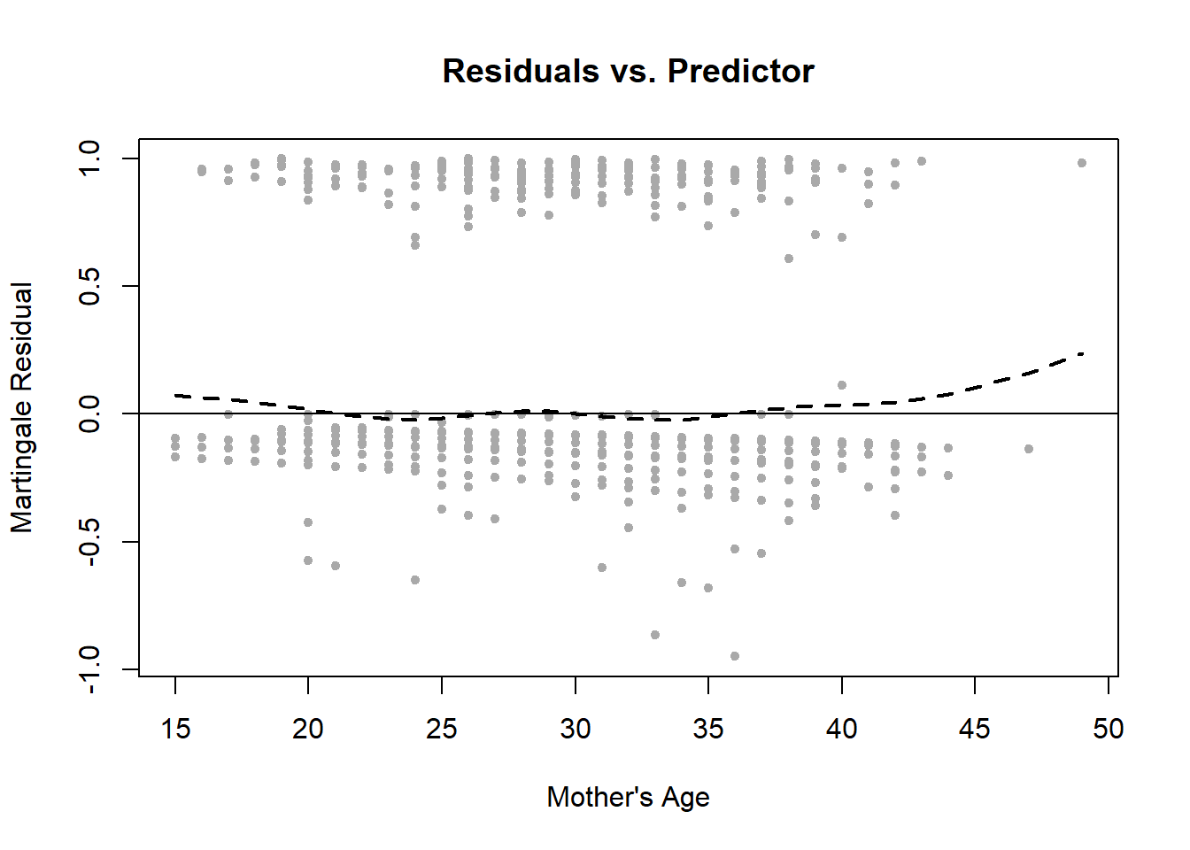

Scatterplot of martingale residuals vs. mother's age with a smoother that looks curved

Figure 7.20: Visually assessing the linearity assumption of a Cox regression

The residuals vs. mother’s age curve appears somewhat non-linear. As with other regression models, to relax the linearity assumption, transform the predictor using a polynomial, logarithm, or other function. The code below adds a quadratic term for maternal age and re-checks the linearity assumption (Figure 7.21).

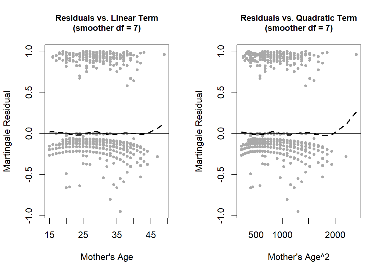
Scatterplots of martingale residuals vs. mother's age and mother's age squared, each with a smoother that only deviates from linear at the extreme where there is little data

Figure 7.21: Re-checking the linearity assumption after adding a quadratic term

As shown in Figure 7.21, adding a quadratic term helps with the non-linearity (the uptick in the curves at older maternal age is due to a single observation with an extreme age value). Inside of smooth.spline(), change df to a smaller (larger) value to get more (less) smoothing. In Figure 7.22, the plots with df = 3 appear linear at all ages.

Same as the previous residual vs. predictor plots but this time with more smoothing so there is no deviation from linear

Figure 7.22: Changing the amount of smoothing when checking the linearity assumption

In general, be careful when using a small df value; make sure to also look at the plot with a larger df value, as we did here, to make sure you are not over-smoothing.