5.5 Visualizing the unadjusted relationships

Before fitting the model, visualize the association between the outcome and each predictor. These plots will not correspond exactly to the MLR model since they will not be adjusted for any other predictors, but they are a useful place to start just to make sure the predictors you are using are what you think they are (if the plot looks very strange, go back and look at your code to make sure you are using the variables you want to use and that they were coded correctly). Later, in Section 5.8, we will examine plots that are adjusted for the other predictors in the model.

Example 5.1 (continued): Plot the relationship between fasting glucose (LBDGLUSI) and each of waist circumference (BMXWAIST), smoking status (smoker), age (RIDAGEYR), gender (RIAGENDR), race/ethnicity (RIDRETH3), and income, one predictor at a time. The plots are shown in Figure 5.3.

You could use the code found in Section 4.1 to create each plot one at a time. Or, you can use the function plotyx() found in Functions_rmph.R (which you loaded at the beginning of this chapter). Each time you call plotyx(), pass the names of the specific outcome and predictor you are interested in plotting as arguments to the function. As a preliminary step, the code below makes copies of the race/ethnicity and income variables with shorter labels so they will fit in the plot.

# Rename the levels with shorter labels that fit in the plot
levels(nhanesf.complete$race_eth)

## [1] "Hispanic"           "Non-Hispanic White" "Non-Hispanic Black" "Non-Hispanic Other"

nhanesf.complete$race_ethb <- nhanesf.complete$race_eth
levels(nhanesf.complete$race_ethb) <- c("H", "NHW", "NHB", "NHO")

levels(nhanesf.complete$income)

## [1] "<$25,000"            "$25,000 to <$55,000" "$55,000+"

nhanesf.complete$incomeb <- nhanesf.complete$income
levels(nhanesf.complete$incomeb) <- c("<$25K", "$25K-<$55K", "$55K+")

NOTE: The syntax is plotyx("y", "x", data) (outcome first, then predictor, then dataset) where "y" and "x" are character strings naming the variables you want to plot.

# If you have not already loaded this file...
# ...do so now to make plotyx() available
source("Functions_rmph.R")

# Change margins
# Default par(mar=c(5, 4, 4, 2) + 0.1) for c(bottom, left, top, right)
par(mar=c(4.5, 4, 1, 1))
par(mfrow=c(2,3))
plotyx("LBDGLUSI", "BMXWAIST",  nhanesf.complete,
       ylab = "FG (mmol/L)", xlab = "Waist Circumference (cm)")
plotyx("LBDGLUSI", "smoker",    nhanesf.complete,
       ylab = "FG (mmol/L)", xlab = "Smoking Status")
plotyx("LBDGLUSI", "RIDAGEYR",  nhanesf.complete, 
       ylab = "FG (mmol/L)", xlab = "Age (years)")
plotyx("LBDGLUSI", "RIAGENDR",  nhanesf.complete, 
       ylab = "FG (mmol/L)", xlab = "Gender")
# Using race_ethb and incomeb (the versions with shorter labels)
plotyx("LBDGLUSI", "race_ethb", nhanesf.complete, 
       ylab = "FG (mmol/L)", xlab = "Race/Ethnicity")
plotyx("LBDGLUSI", "incomeb",   nhanesf.complete,
       ylab = "FG (mmol/L)", xlab = "Income")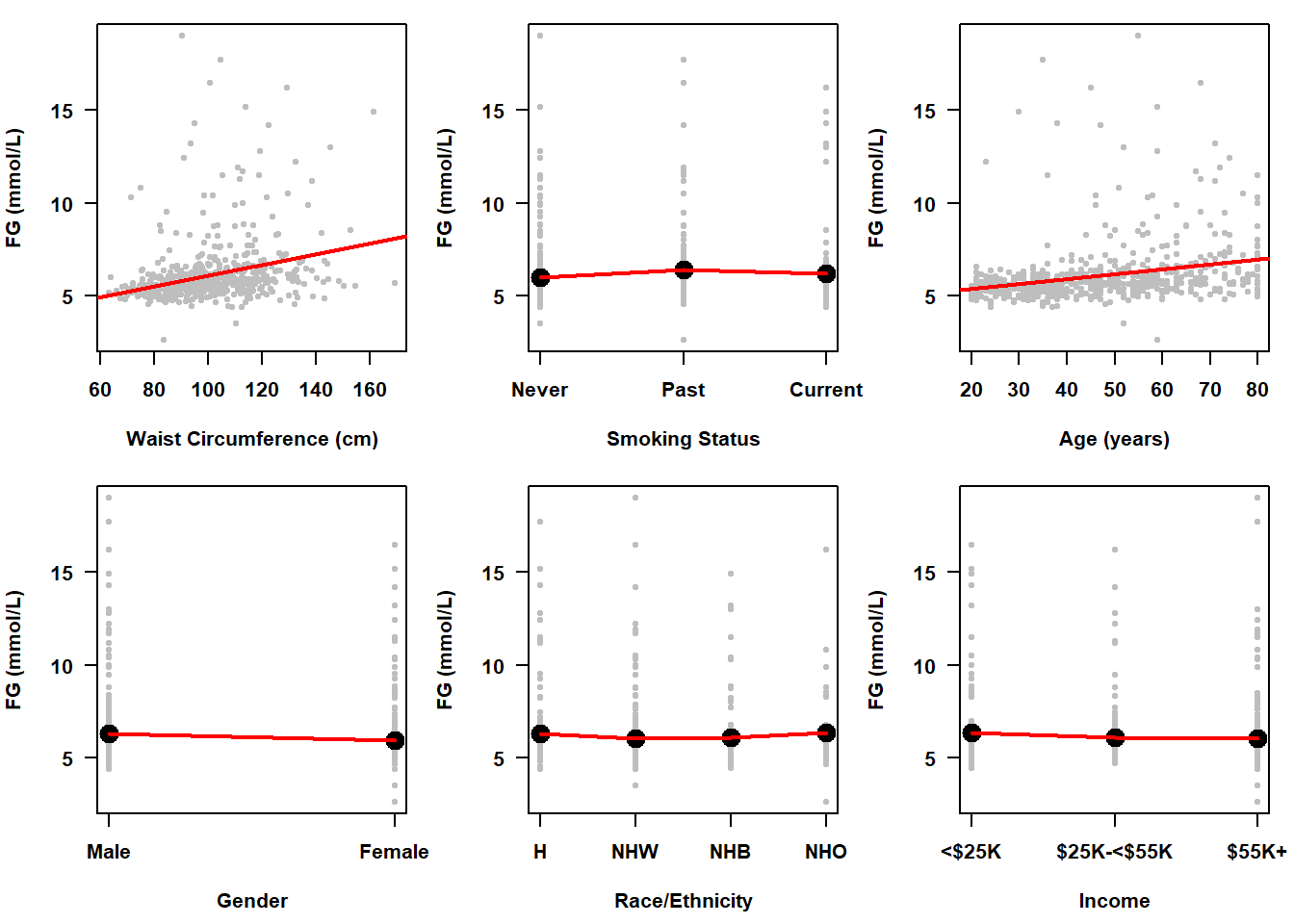

Six scatterplots of fasting glucose vs. waist circumference, smoking status, age, gender, race/ethnicity, and income, each with a regression line

Figure 5.3: Unadjusted associations with fasting glucose (mmol/L)