Chapter 3 RPA Aquired Data and Lidar DEM
Microclimate sites in the Gavin Lake block were surveyed with a RPA between June 28th and July 4th, 2020. The 10 microclimate plots were flown in four different flight areas. Flights used a DJI Phantom 4 RTK and DJI Pro software for flight planning. DAP and orthophotos are produced from flights with optimum cloudy conditions. Flight heights depended on a field assessment of a safe distance from treetops and ranged from 70 m to 120 m above ground. For the canopy height models, I used the lowest elevation flight data. Details of the RPA, camera and flight planning are included in the table below
| Aircraft | |
|---|---|
| Max Flight Time | Approximately 30 mins |
| Navigation | RTK |
| GPS Positional Accuracy | Vert. +/0.1; Horizontal, +/- 0.1 m |
| Transmission Range | 7 km |
| Camera | |
| Sensor | 1” CMOS |
| ISO Range | 100-3200 |
| Electronic Shutter Speed | 1/8000 s |
| FOV | 84 deg |
| Aperture | f/2.8 |
| Image Size | 4864 x 3648 |
| Acquisition Parameters | |
| Altitude | ~70 m (AGL) |
| Terrain Following | 15 m (ALS) |
| Image Overlap | 90 % forward, 80% lateral |
3.1 Raw photos and flight details
Ground Control Points
Flight areas are defined by the relative elevation, upper, middle, lower, and one plot called “Old Guy.” Raw photos a seperated by 1). flight area and 2) flight. All plots had three seperate flights. Distance above ground is variable but is noted in the file naming schema (e.x. 70m)
Each flight area also at least 5 ground control points that were deployed at some point. Ground control points are here. The naming convention denotes the flight area, the GCP # and the locations of the closest microclimate logger. File locations are shown in Table 3.1
ground_control_points <- read.csv('_RPA-Aqcuired-Data/Flights/Ground_ControlPts/gc_pts_accuracy_CORRECT_WGS84.csv')
head(ground_control_points)
## X name lat long hght XYAccuracy
## 1 1 topplotsgc12ct7 52.45502 -121.7431 1089.157 0.014431
## 2 2 topplotsgc10ct3 52.45550 -121.7427 1102.296 0.008229
## 3 3 topplotsgc9ct9-8 52.45585 -121.7423 1108.561 0.011566
## 4 4 topplotsgc8ct1-2 52.45632 -121.7427 1101.110 0.011921
## 5 34 upperplotsgc13 52.45525 -121.7401 1142.658 0.007607
## 6 38 upperpotsgc1 52.45498 -121.7405 1140.914 0.009394Flight Photos
| Flight_Area | Flights |
|---|---|
| D:/Data/SmithTripp/SmithTripp_Metadata/_RPA-Aqcuired-Data/Flights/Ground_ControlPts | gc_pts_accuracy_CORRECT_WGS84.csv |
| D:/Data/SmithTripp/SmithTripp_Metadata/_RPA-Aqcuired-Data/Flights/LowerPlots | 0626_120m_LowerPlots |
| 0628_100m_LowerPlots_1 | |
| 0628_100m_LowerPlots2 | |
| 0705_70m_LowerPlots | |
| D:/Data/SmithTripp/SmithTripp_Metadata/_RPA-Aqcuired-Data/Flights/Midplots | 0629_MidPlots_70m_1 |
| 0629_MidPlots_70m_2 | |
| 0629_MidPlots_90m | |
| D:/Data/SmithTripp/SmithTripp_Metadata/_RPA-Aqcuired-Data/Flights/OldGuy | 0628_100m_OldGuy_1 |
| 0628_100m_OldGy_2 | |
| 0628_90m_OldGuy | |
| 0704_70m_OldGuy | |
| D:/Data/SmithTripp/SmithTripp_Metadata/_RPA-Aqcuired-Data/Flights/Upperplots | Upperplots_part1_03-July-2020_80m |
| Upperplots_part1_03-July-2020_90m | |
| Upperplots_part1_03July2020_70m_partialflight | |
| Upperplots_part1_06-29-20_80_2 | |
| Upperplots_part1_06-29-20_80m | |
| Upperplots_part1_06-29-20_90m | |
| UpperPlots_part2_04July2020_70m | |
| Upperplots_part2_06-30-20_100m | |
| Upperplots_part2_06-30-20_90m |
3.2 Processed DAP point clouds
Digital Surface Models Digital surface models include the ground and the canopy. These have not been normalized. They have been aligned to 2009 lidar point clouds. The accuracy of ICP and metashape photo alignment is noted in Table 3.2. This excel file has the transformation matrix applied to the clouds to align to lidar.
## New names:
## * `` -> ...3| Flight Area | Program | …3 | Analysis Type | Value |
|---|---|---|---|---|
| Lower Plots | MetaShape | RTK | RMS | 0.285763 |
| Photo | Included RMS | 0.851225 | ||
| Check RMS | 2.247132 | |||
| Cloud Compare | ICP | RMS | 1.584300 | |
| Mean Pt. Cloud Distance | 1.008540 | |||
| St. Dev Cloud Distance | 0.697100 |
Point clouds included in this meta-data are both aligned but not normalized to the lidar DEM. Align these to the lidar DEM, evaluate the code below:
library(lidR)
# List files
aligned_las <- list.files(paste0(getwd(),"/_RPA-Aqcuired-Data/DAP_Point_Clouds/Point_Clouds/Non-classified"))
#read LAS files
aligned <- lapply(aligned_las, readLAS)

#load DEM to normalize las files
dem <- raster("_RPA-Aqcuired-Data/Lidar_DEM/clip_DEM.tif")

#normalize all point clouds with 1-m Lidar DEM
normalized <- lapply(aligned, normalize_height, dem)

 #write function to change all returns to first return (because DAP point cloud)
convert_return <- function(las){
  las@data$ReturnNumber <- 1
  return(las)
}
#convert all returns to 1 for DAP data
normalized_1 <- lapply(normalized, convert_return)
3.3 Canopy Structure Rasters
Canopy Structure Rasters are divided into Canopy height and cover models with a 10cm resolution and Canopy Structural Metrics also at 10cm. A list of all canopy structural metrics is included in Table 3.3 Canopy Structure.
All details of the the processing for the canopy height raster are included in the “Canopy_Model_Processing.R” file.
| Flight_Area | Flights |
|---|---|
| D:/Data/SmithTripp/SmithTripp_Metadata/_RPA-Aqcuired-Data/Canopy_Structure/Canopy_Cover | lower_plots_canopycov.tif |
| midplots_canopycov.tif | |
| oldguy_canopycov.tif | |
| UpperPlots_canopycov.tif | |
| D:/Data/SmithTripp/SmithTripp_Metadata/_RPA-Aqcuired-Data/Canopy_Structure/Canopy_Height | lower_plots_chm_10cm.tif |
| midplots_chm_10cm.tif | |
| oldguy_chm_10cm.tif | |
| UpperPlots_chm_10cm.tif | |
| D:/Data/SmithTripp/SmithTripp_Metadata/_RPA-Aqcuired-Data/Canopy_Structure/Canopy_Metrics | lower_plots_metrics.tif |
| midplots_metrics.tif | |
| oldguy_metrics.tif | |
| UpperPlots_metrics.tif | |
| D:/Data/SmithTripp/SmithTripp_Metadata/_RPA-Aqcuired-Data/Canopy_Structure/Canopy_Model_Processing.R | |
| D:/Data/SmithTripp/SmithTripp_Metadata/_RPA-Aqcuired-Data/Canopy_Structure/Tree_Locations | Lower_plots |
| MidPlots | |
| OldGuy | |
| Topplots |
3.4 Lidar DEM Rasters
I include the DEM I used for my analyses and the raw point file. The lidar point cloud has a point density of 5 pts/m^2. For more information see (Coops, Duffe, and Koot 2010)
## [1] "D:/Data/SmithTripp/SmithTripp_Metadata/_RPA-Aqcuired-Data/Lidar_DEM/clip_DEM.tif"
## [2] "D:/Data/SmithTripp/SmithTripp_Metadata/_RPA-Aqcuired-Data/Lidar_DEM/gavin_lake_all.las"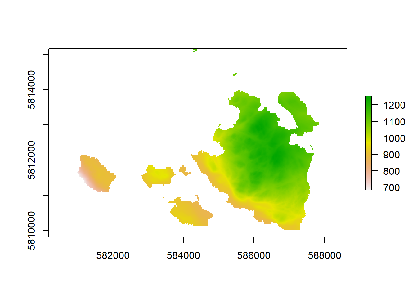
References
Coops, Nicholas C., Jason Duffe, and Cathy Koot. 2010. “Assessing the Utility of Lidar Remote Sensing Technology to Identify Mule Deer Winter Habitat.” Canadian Journal of Remote Sensing 36 (2): 81–88. https://doi.org/10.5589/m10-029.