4 Linear Regression
Linear regression is one of the most fundamental statistical techniques in science and data science. It’s fast, generally simple, and applicable to a range of problems. All of you have learned regression in some form or another in order to take this class, but because it’s so universal we’re still going to go over again. So, if you already are solid with regression, hopefully you’ll reinforce your knowledge and learn a few tricks. If you’re newer to it I hope this gives you a change to really learn the guts of it.
4.1 A quick note on the structure of this lesson
We’re going to be manually calculating all the critical parameters and estimates associated with regression models. This is tedious, but the point is for you to truly understand the math underlying them. Doing so will allow you to develop an intuitive understanding of their interrelationships and how they should influence your interpretation and confidence of your model. Thus, you should be running the code within in your own R console and playing with the data and code along the way. Want to see what happens to the residual standard error estimate when you increase sample size? Go ahead and modify our simulation and see how that influences your calculations! Want to determine how decreasing variation in our simulation population affects our \(R^2\)? Modify the code and find out! Finally, at the end I encourage you to play with a more interactive regression simulator that I made.
This lesson is divided into a two sections.
Understanding how a regression model is fit & calculating various fit statistics
Making inference from regression models and extending the to multiple features and feature types
4.2 Understanding how a regression model is fit
4.2.1 What’s the goal of regression?
In its most basic form, the goal of linear regression is to determine how a single feature relates to a target or response. Target and response variables refer to the same thing, although I find that academics and statisticians tend to say response and data scientists say target (I’ll be using target). These relationships are everywhere. For example:
- How does height relate to weight of a human?
- How does the amount of money spent on advertising relate to sales?
- How does the square footage of a house relate to its price?
Linear regression assumes a linear relationship between these targets (what you’re trying to predict) and features (what you’re using to predict the target). In other words, for every unit your feature increases, you’d see a proportional change in the target. In the context of our examples above this could be something like:
- For every 1 inch taller a person gets they weigh 8 pounds more.
- For every $100 spent on advertising a company sells 50 more units of a product.
- For every 100 extra square feet in a house the value increases by $10,000.
Of course, maybe increasing spending on advertising from $1000 to $1100 may increase sales by 50 units, but increasing from $10,000 to $10,100 may only increase sales by 5 units. In that case the relationship is not actually linear, but it might not be a big deal if we still assume it’s linear.
4.2.2 Looking at the regression formula
OK, so we assume that there is a relationship between our feature and target, but how do we actually figure out what that relationship is? What exactly is R doing to calculate those values? We’ll, let’s consider the actual formula for linear regression: \[y = \beta_0 + \beta_1x + \epsilon\] Of course, our target is \(y\) and our feature is \(x\) with some error term \(\epsilon\). So the question is how do we determine what intercept (\(\beta_0\)) and slope (\(\beta_1\)) best describe the linear relationship between target and feature? Well, you want to find values that allow your estimated y values (which we’ll name \(\hat{y}\)) to be as close as possible to our actual \(y\) values. Let’s generate some data to start illustrating how this is done.
Here’s a quick function that allows us to generated simulated height - weight relationships without having crazy unrealistic values (e.g. weights below 85lbs). You don’t have to know what’s going on in detail. Just know that if you copy it into your console and run it you’ll then have the function available to use.
ht_wt_sim <- function(num_samples, std_dev) {
 height <- runif(num_samples, min = 60, max = 75) # generate random heights
 noise <- rnorm(num_samples, sd = std_dev) # generate error
 weight <- height*7.6 - 355 + noise # create relationship with target
 for(i in 1:length(weight)){
  if(weight[i] <= 85) {
   weight[i] <- runif(1, min = 85, max = 120)
  } else if (weight[i] >= 350) {
   weight[i] <- runif(1, min = 180, max = 300)
  }else {
   weight[i] <- weight[i]
  }
 } # deal with weird values
 df <- data.frame(height = height,
          weight = weight) # put in df
 return(df)
}
Let’s generate some data with our function. We input the desired sample size and standard deviation.
ht_wt <- ht_wt_sim(num_samples = 30, std_dev = 20)
ht_wt <- round(ht_wt) # round it too
Always look at your data! In this case just using head() does the trick.
| height | weight |
|---|---|
| 72 | 188 |
| 63 | 141 |
| 75 | 219 |
| 63 | 112 |
| 65 | 158 |
| 71 | 172 |
Plotting our data gives us this. So there’s obviously a linear relationship there, but how do we actually fit our line? What’s our intercept and slope that minimizes the difference between our fitted target values (\(\hat{y}_i\)) and our actual \(y_i\) values?
ggplot(ht_wt,
    aes(x = height, y = weight)) +
 geom_point() +
 theme_classic() +
 theme(text = element_text(size = 20))
Thus, we want the total smallest value when we add up the difference between the actual value and fitted value for each observation in our dataset. In other words, we want to minimize: \[\sum_{x = 1}^{n} (\hat{y}_i - y_i)^2 = RSS\] We square the difference between fitted target values (\(\hat{y}_i\)) and our actual \(y_i\) values to keep everything the same sign. This is known as the Residual Sum of Squares or \(RSS\). Visually, you can see in the figure below that our RSS would be the same as summing up every purple segment. You could imagine those purple lines getting longer and longer if the line flattened out or became more vertical, thus increasing the \(RSS\) and worsening the fit.
## `geom_smooth()` using formula 'y ~ x'
To find our \(\beta_1\) and \(\beta_0\) values that minimize our \(RSS\) we can use some calculus… but the actual math is outside the scope of this course so we’re going to skip it. After the calculus you get two formulas for finding \(\beta_1\) and \(\beta_0\) \[\hat{\beta}_1 = \frac{\sum_{i = 1}^n (x_i - \overline{x})(y_i - \overline{y})} {\sum_{i = 1}^n (x_i - \overline{x})^2}\]
And our \(\beta_0\) is easy once we have our \(\beta_1\)
\[\hat{\beta}_0 = \overline{y} - \hat{\beta}_1\overline{x}\]
So when you fit a linear regression model using ordinary least squares, this is how it’s being done. Of course, you can just go and use lm(weight ~ height, data = ht_wt) to do that, but what’s the fun in that? Let’s actually manually calculate our \(\beta_1\) and \(\beta_0\)
4.2.3 Calculating \(\beta_1\) and \(\beta_0\) from scratch
Let’s break this into chunks and follow the formula above. Remember we’re trying to figure the relationship between height (our feature \(x\)) and our weight (our target \(y\)). You can call say \(x_i\) by calling the column from the data frame(in this case ht_wt$height). Also remember that a bar over a variable (e.g. \(\overline{x}\)) is indicating that that’s the mean for that variable. You can just use the mean() function on the column (say mean(ht_wt$height)) to calculate it.
b1_num <- sum( (ht_wt$height - mean(ht_wt$height)) *
         (ht_wt$weight - mean(ht_wt$weight)) ) # numerator first
b1_denom <- sum((ht_wt$height - mean(ht_wt$height))^2) # now denominator
b1 <- b1_num / b1_denom # divide per the formula
What’s our calculated \(\hat\beta_1\) estimate?
## [1] 8.591714And get our \(\beta_0\) quick
b0 <- mean(ht_wt$weight - b1 * mean(ht_wt$height))
b0
## [1] -420.8524Let’s now use R’s lm(function) to fit a model, store it to an object, and look at a summary.
ht_wt_model <- lm(weight ~ height, data = ht_wt) # fit model store as object
ht_wt_model_summary <- summary(ht_wt_model) # store summary to object
ht_wt_model_summary # check out the summary object
##
## Call:
## lm(formula = weight ~ height, data = ht_wt)
##
## Residuals:
## Min 1Q Median 3Q Max
## -37.751 -10.930 -4.588 10.728 37.616
##
## Coefficients:
## Estimate Std. Error t value Pr(>|t|)
## (Intercept) -420.8524 46.5426 -9.042 8.46e-10 ***
## height 8.5917 0.6938 12.384 7.06e-13 ***
## ---
## Signif. codes: 0 '***' 0.001 '**' 0.01 '*' 0.05 '.' 0.1 ' ' 1
##
## Residual standard error: 19.01 on 28 degrees of freedom
## Multiple R-squared: 0.8456, Adjusted R-squared: 0.8401
## F-statistic: 153.4 on 1 and 28 DF, p-value: 7.058e-13Cool! So although it may seem like magic at times, the actual math underlying how linear regression models are fit using OLS is actually relatively simple. We can see that the intercept and slope of the fitted model exactly match our manually calculated \(\beta_0\) and \(\beta_1\) values, as they should!
4.2.4 Understanding quality of fit
Obviously our \(\hat{\beta}_0\) and \(\hat{\beta}_1\) are estimates of the true \(\beta_0\) and \(\beta_1\). While normally you don’t know the true values (that’s why you’re fitting the model!) but in this case we actually do as we simulated the data. Looking back at the function we used to generate the data we can see the true values weight <- height*7.6 - 355 + noise. So although we estimated that for every extra 1 inch in height a person is they weigh 8.59 pounds more, the actual process underlying it is 7.6 pounds for every 1 inch. But this is simulating a natural system where there is variation around the generating process. This takes us to the next key part of this lesson - understanding how good our estimated values actually are at describing the data. In other words, with the estimated \(\hat{\beta}_0\) and \(\hat{\beta}_1\), how close is \(\hat{y}\) (our estimated target) to \(y\) (the observed value) on average?
You can really divide these up into statistical measures that consider the quality of the overall model, and then those that consider the parameters within.
4.2.4.1 Residual Standard Error
For the overall model itself, we can estimate the Residual Standard Error or \(RSE\) (also known as sigma \(\sigma\)). The formula to calculate this is first dividing the \(RSS\) by the sample size \(n\) minus the number of predictors \(p\) and 1. You then take the square root of this: \[RSE = \sqrt\frac{RSS}{n - p - 1} = \sigma \] Stepping back and thinking about \(RSE\) formula for a bit we can see a couple things.
As sample size \(n\) increases, our denominator grows and thus \(RSE\) shrinks. Thus, with more observations we can reduce our estimation error. Go play with the simulator. What happens when you increase samples size?
Conversely, as the number of parameters \(p\) in our model grows, our \(RSE\) will increase. Thus, model complexity (i.e. adding more features) can influence model fit. Let’s go an actually calculate our \(RSE\) value. To start let’s calculate \(RSS\) using the forumula \(RSS = \sum_{x = 1}^{n} (\hat{y}_i - y_i)^2\). Note that this needs both our observed \(y\) values and the associated estimated \(y\) values (aka \(\hat{y}\)). Thus, let’s calculate each \(\hat{y}_i\) for each \(x_i\) using our previously calculated \(\hat{\beta}_0\) and \(\hat{\beta}_1\):
y_hat <- b0 + b1*ht_wt$height
y_hat # let's look at our estimated weights
## [1] 197.7511 120.4256 223.5262 120.4256 137.6091 189.1594 223.5262 154.7925
## [9] 94.6505 129.0174 197.7511 94.6505 103.2422 111.8339 120.4256 197.7511
## [17] 103.2422 206.3428 154.7925 154.7925 223.5262 171.9759 103.2422 111.8339
## [25] 197.7511 129.0174 103.2422 171.9759 163.3842 206.3428So now we have estimated weights (\(\hat{y}_i\)) for every height observation (\(x_i\)). We can now calculate our \(RSS\) step by step:
difference <- y_hat - ht_wt$weight # difference between estimated and real weights
diff_square <- difference ^ 2 # square each of them
RSS <- sum(diff_square) # sum them to get RSS
RSE <- sqrt(RSS / (nrow(ht_wt) - 1 - 1)) # use RSE formula
RSE #check RSE aka sigma
## [1] 19.00848Boom! Our model summary that R fit using lm() shows the exact same RSE as our manual calculation.
ht_wt_model_summary$sigma # checking RSE from our earlier model summary ## [1] 19.00848In plain English, our \(RSE\) is telling us that on average our weight estimates are going to be off by 19.01lbs. Can you go back and modify our simulated data to have a higher standard deviation? What does this do to our estimates throughout?
4.2.4.2 What about \(R^{2}\) values?
\(RSE\) is a great way to figure out how accurate your model is at describing the underlying process, but there’s more that we need to consider. Specifically, we often want to know how much of the total variation we’re explaining. To do this we will calculate the \(R^{2}\) value, which allows us to assess the proportion of variation we’re accounting for. Values close to 1 means our feature (weight) is able to explain nearly all the variation in the target (height). Close to 0 means we’re not explaining much. We really only need to know two things to calculate our \(R^{2}\) value:
The amount of variation in our target (weight) that our model doesn’t explain - Luckily this is what the \(RSS\) is!
The total amount of variation in our target in general.
We quantify the total variation in the target by calculating the Total Sum of Squares AKA \(TSS\) as follows: \[TSS = \sum_{i = 1}^{n}(y_i - \overline{y})^2\] Thus, closer each height is to the average height in the sample, the smaller the \(TSS\). Now, if everyone’s height is very different, then \(TSS\) will be large.
Given \(R^2\) is the proportion of variation explained, we divide how much variation in the \(TSS\) isn’t explained by the \(RSS\) and divide that by the total \(TSS\). \[R^2 = \frac{TSS - RSS}{TSS}\] Let’s just think for a second about how this relates to model fit. Good models will have a really low \(RSS\) as they explain most of the variation, and thus \(TSS - RSS\) will be very close to just \(TSS\). Dividing the two will be nearly 1, meaning that our model explains almost all the variation (as it should since there’s little error!). Now, poor models will have high \(RSS\), so the numerator will become small with a large denominator and thus small \(R^2\).
Let’s calculate \(R^2\)
#First TSS
difference_from_mean <- ht_wt$weight - mean(ht_wt$weight)
difference_from_mean_squared <- (difference_from_mean)^2
TSS <- sum(difference_from_mean_squared)
R2 <- (TSS - RSS) / TSS
R2
## [1] 0.8456167Success! So we also manually calculated our \(R^2\) values and they matched lm().
ht_wt_model_summary$r.squared## [1] 0.8456167So does this \(R^2\) actually mean? Well, it’s saying that just the feature height explains 84.56% (\(R^2\) converted to a percent) of the variation in height we observe in the population. Thus, you can pretty objectively say that it’s a useful model. This is in a lot of ways better than just using the RSE interpreting the RSE is tricky without knowing something about the targets and features as well as having something to compare it to.
4.2.4.3 Confidence Intervals for Features
Our \(RSE\) and \(R^2\) values are great for describing the overall usefulness of the model, and will become critical for when we start comparing multiple models. But what about the features within the model? For now we just have one feature, height, but what if we had others such as sex, age, activity level, etc.? How would we determine which ones also have an effect, and if that effect is real. After all, we saw that our estimated \(\hat{\beta}_1\) at 8.59 differed from our true \(\beta\) of 7.6. Is this difference something to be concerned about? That’s where confidence intervals come in! Confidence intervals will allow us to take into account the amount of variation in the feature to determine how confident we should be in the direction of our estimated slope.
Although the formula for confidence intervals is a bit complex, it doesn’t use anything we haven’t already calculated. To get the confidence interval we first calculate the standard error associated with \(\hat{\beta}_1\), and then the confidence interval. To get the standard error we use: \[SE(\hat{\beta}_1)^2 = \frac{\sigma^2}{\sum_{i = 1}^{n}(x_i - \overline{x}_i)^2}\] Two things I want you to see when looking at this formula.
We already estimated our overall RSE which is \(\sigma\), which we can obviously just square to get \(\sigma^2\). Thus, the larger the RSE of the model, the larger the SE of the parameters within. Makes sense.
Variation in your feature matters for estimation. As the spread of points around \(x\) increases, your denominator grows and thus \(SE\) shrinks… so it’s easier to get an accurate estimate of \(\hat{\beta}_1\) then. Look at the two graphs below. Both were generated with our simulator above, but one is restricted to a narrower range of heights. Just visually it makes sense that it would be easier to estimate the slope for the graph on the left than right, right? This is why having variation to estimate on is important.
## Warning: Removed 11 rows containing missing values (geom_point).## Warning: Removed 2 rows containing missing values (geom_point).
OK, so let’s apply the formula to calculate \(SE(\hat{b}_1)^2\)
# let's just calculate the various components individually
sigma_2 <- RSE^2 # use RSE to get variance (sigma squared)
x_mean_diff_squared <- (ht_wt$height - mean(ht_wt$height))^2
sum_x_mean_diff_squared <- sum(x_mean_diff_squared)

SE_b1_squared <- sigma_2 / sum_x_mean_diff_squared # calculate
SE_b1 <- sqrt(SE_b1_squared) #remember to take square root!
SE_b1
## [1] 0.693768Nice, so our calculated standard error of \(\hat{\beta}_1\) matches what lm() calculated.
ht_wt_model_summary##
## Call:
## lm(formula = weight ~ height, data = ht_wt)
##
## Residuals:
## Min 1Q Median 3Q Max
## -37.751 -10.930 -4.588 10.728 37.616
##
## Coefficients:
## Estimate Std. Error t value Pr(>|t|)
## (Intercept) -420.8524 46.5426 -9.042 8.46e-10 ***
## height 8.5917 0.6938 12.384 7.06e-13 ***
## ---
## Signif. codes: 0 '***' 0.001 '**' 0.01 '*' 0.05 '.' 0.1 ' ' 1
##
## Residual standard error: 19.01 on 28 degrees of freedom
## Multiple R-squared: 0.8456, Adjusted R-squared: 0.8401
## F-statistic: 153.4 on 1 and 28 DF, p-value: 7.058e-13Last step… let’s use our \(SE\hat{\beta}_1\) to calculate the 95% confidence interval. The formula is simple just adding/subtracting 2 x our \(SE(\hat{\beta}_1)\) from \(\hat{\beta}_1\): \[\hat{\beta}_1 \pm 2 \cdot SE(\hat{\beta}_1)\] Let’s calculate
b1_ci_upper <- round(b1 + 2*SE_b1, 2) # round to 2 places for clarity
b1_ci_lower <- round(b1 - 2*SE_b1, 2)
paste('Our confidence interval is from', b1_ci_lower, 'to', b1_ci_upper)
## [1] "Our confidence interval is from 7.2 to 9.98"Why do we care about our confidence interval? We’ll, it’s telling us that 95% of the time the true effect of weight on height will be between 7.2 and 9.98. The key thing here is that if your confidence interval ends up encompassing zero, then you are not 95% confident that your slope is strictly positive or negative. Thus, it’s not statistically different from a simple flat line. Clearly our 95% confidence encompasses our \(\hat{\beta}_1\) estimate of 8.5917144, so we’re statistically confident of the estimated relationship of height being positively related to weight.
You can calculate the 95% confidence interval for \(\hat{\beta}_0\) using these two formulas, but I’ll leave that all up to you! \[SE(\hat{\beta}_0)^2 = \sigma^2 \left[\frac{1}{n} + \frac{\overline{x}^2}{\sum_{i = 1}^{n}(x_i - \overline{x}_i)^2}\right]\] \[\hat{\beta}_0 \pm 2 \cdot SE(\hat{\beta}_0)\]
4.2.4.4 \({p}\)-values
Probably the worst metric for assessing models are \(p\)-values (in my stubborn opinion). This is for a number of reasons, but probably the biggest one is that they encourage a binary style of thinking when it comes to parameter importance. Often, people see a p < 0.05 and say, oh, this matters. And sure, that’s not false, but also we know that the effects of different things could vary, and we should understand how much of an effect a feature has on explaining our target, rather than just saying yes/no. Also, the \(p\)-value threshold of 0.05 is pretty arbitrary. Are you really going to say confidently that a feature with a p = 0.052 doesn’t matter while a feature with a \(p\) = 0.048 does? No, that would be crazy. Thus, although I don’t think they’re evil, I generally encourage a more holistic assessment of a model (see everything above) rather than just using \(p\)-values!
Hypothesis testing should be a core idea within data science. After all, it is supposed to be science. At its basic form hypothesis testing puts forward the idea that you have a null and alternative hypothesis as follows:
\[H_0 = \text{The feature of interest has no effect on the target}\] \[H_1 = \text{The feature of interest does have an effect on the target}\] When you perform a hypothesis test you’re testing if \(H_0\) is true or not. If it is, then you say there’s no relationship. If it’s not, then you say ‘we reject \(H_0\) and accept \(H_1\). This gets into some tricky logic that statisticians argue over as you actually aren’t testing \(H_1\), but we’re going to avoid that discussion here. The key thing is that you should be thinking deeply about what you’re actually asking. What are your \(H_0\) and \(H_1\)? Does your model actually test them? Can you data actually test them? The book explores how to calculate \(p\)-values, so I’ll allow you to explore that on your own. For the purpose of the class we’re going to use a threshold of \(p\) < 0.05 is ’significant’
If we look at our model summary we see that \(p\)-values are calculated automatically when we fit a model with lm(). The column \(Pr(>|t|)\) contains them. We can see that the p-value for the effect of our feature height on our target weight is 0 and thus would be deemed significant… but this isn’t surprising as we already know the 95% confidence interval comes nowhere near encompassing zero, and so of course it’s significant. Go play with the simulator. Do you ever find the CI overlapping zero while the p-value is significant?
ht_wt_model_summary##
## Call:
## lm(formula = weight ~ height, data = ht_wt)
##
## Residuals:
## Min 1Q Median 3Q Max
## -37.751 -10.930 -4.588 10.728 37.616
##
## Coefficients:
## Estimate Std. Error t value Pr(>|t|)
## (Intercept) -420.8524 46.5426 -9.042 8.46e-10 ***
## height 8.5917 0.6938 12.384 7.06e-13 ***
## ---
## Signif. codes: 0 '***' 0.001 '**' 0.01 '*' 0.05 '.' 0.1 ' ' 1
##
## Residual standard error: 19.01 on 28 degrees of freedom
## Multiple R-squared: 0.8456, Adjusted R-squared: 0.8401
## F-statistic: 153.4 on 1 and 28 DF, p-value: 7.058e-134.2.4.5 \(F\)-statistic
\(F\)-statistics provide a way to get a \(p\)-value for the entire model. The larger the \(F\) value the smaller the \(p\)-value. While the entire model’s \(p\)-value is the same when there is only one feature, that is not the case when you have many features. Essentially the whole model \(p\)-value will ask if at least one \(\beta\) coefficient has a significant \(p\)-value.
We can calculate \(F\) using our \(TSS\) and \(RSS\) as follows: \[F = \frac{(TSS - RSS) / p}{RSS/(n - p - 1)}\] You can then use \(F\) to get a \(p\)-value. I’ll let you figure out how to do that on your own. Instead, I want to think about the following things and how a large F leads to higher confidence (and a smaller \(p\)-value).
The larger the \(RSS\), and thus the less of the \(TSS\) you’re explaining, the larger the denominator is and thus larger the F.
The larger the sample size \(n\) the smaller the denominator, and thus the larger the \(F\) this is why it’s easier to detect significant effects even with lots of noise when you have a large sample size.
The more parameters the smaller your \(F\), and thus more complex models can have smaller \(F\) stats than simpler ones. This won’t matter much for one or two parameters, but if you have many parameters \(p\) and a relatively small sample size \(n\) then you can run into problems!
Let’s calculate \(F\):
f_num <- (TSS - RSS)/1 #p = 1 as only one parameter
f_denom <- RSS/(nrow(ht_wt) - 1 - 1)
f_stat <- f_num/f_denom
f_stat
## [1] 153.3667And verifying from our lm() model summary
ht_wt_model_summary$fstatistic## value numdf dendf
## 153.3667 1.0000 28.0000Great! So hopefully you see how all these model statistics are really just calculated from a few simpler ones that try to understand how much variation our model is explaining. In general, you want to consider all of these numbers together as only considering a single one can lead to a serious over or underestimation of what the data is telling you.
4.3 Linear regression to multiple regression - When there’s more than one feature
Now that we’ve gone into extra detail regarding how linear regression models are fit and assessed, let’s apply our knowledge to a new set of data. Let’s also start considering what happens when you have more than one feature or various types of features. This extends linear regression to Multiple Regression.
We’re going to be using a dataset on insurance costs for individuals who vary in several different parameters. The goal is to figure out the biggest factors that contribute to total medical costs.
Of course, this sets up a challenge… Which parameters hurt model fit? Which ones help? Which ones are most important? Do they interact? How do we answer these questions? Well, we use the all test statistics we learned earlier!
4.3.1 Import and Exploration
As always, import and then explore your data. Bringing in our data as the object costs shows that there are 7 columns and 1338 observations. Obviously we have charges as our target and the rest as features. Thus, this will be a case of multiple regression as there are many features which may or may not help our understanding.
costs <- read_csv("https://docs.google.com/spreadsheets/d/1WUD22BH836zFaNp7RM5YlNVgSLzo6E_t-sznxzjVf9E/gviz/tq?tqx=out:csv")## Parsed with column specification:
## cols(
## age = col_double(),
## sex = col_character(),
## bmi = col_double(),
## children = col_double(),
## smoker = col_character(),
## region = col_character(),
## charges = col_number(),
## bodyfat = col_double()
## )Histograms of our numeric columns make sense overall and I don’t see anything that looks like an erroneous outlier. I will say now that our target, charges, should probably be log transformed, but we’re going to skip that for this lesson.
p1 <- ggplot(costs, aes(x = charges)) + geom_histogram()
p2 <- ggplot(costs, aes(x = bmi)) + geom_histogram()
p3 <- ggplot(costs, aes(x = age)) + geom_histogram()
p4 <- ggplot(costs, aes(x = bodyfat)) + geom_histogram()

plot_grid(p1,p2,p3,p4, ncol=2)
And what values are present in our character columns? Pretty much as expected. We’ll ignore region for this lesson.
unique(costs$sex)## [1] "female" "male"unique(costs$smoker)## [1] "yes" "no"4.3.2 Comparing three regression models
Let’s start by comparing two simple linear regression models. The first will use bmi, or body mass index, as a feature. The second will use age as a feature.
4.3.2.1 Fitting your models
To fit a linear model in R you use the function lm with the syntax lm(TARGET ~ FEATURE, data = YOUR_DATA_FRAME). You should generally assign your model to an object so you can call it up later. Names should be informative so you know that the object is a model and what feature(s) it’s using. Ok, let’s fit the two.
bmi_mod <- lm(charges ~ bmi, data = costs) # call this bmi_mod for clarity
age_mod <- lm(charges ~ age, data = costs) # age_mod for age model
Looking at our charges ~ cost model
R has a function summary() that you can call on a variety of objects, including regression models. You can either call summary directly on a model or store the output as an object. We’ll just do the former for now.
Starting with our model using bmi as a feature.
##
## Call:
## lm(formula = charges ~ bmi, data = costs)
##
## Residuals:
##    Min     1Q Median     3Q    Max
## -20956  -8118  -3757   4722  49442
##
## Coefficients:
##             Estimate Std. Error t value Pr(>|t|)
## (Intercept)  1192.94    1664.80   0.717    0.474
## bmi           393.87      53.25   7.397 2.46e-13 ***
## ---
## Signif. codes:  0 '***' 0.001 '**' 0.01 '*' 0.05 '.' 0.1 ' ' 1
##
## Residual standard error: 11870 on 1336 degrees of freedom
## Multiple R-squared:  0.03934,	Adjusted R-squared:  0.03862
## F-statistic: 54.71 on 1 and 1336 DF,  p-value: 2.459e-13
We see the following things:
Our \(RSE\) is 11870 (FYI, the actual value is 1.1874^{4} that R rounds for some reason), which doesn’t mean much until we start comparing it to other models.
Our Adjusted \(R^2\) value is 0.0393, which means our effect, BMI, is only explaining 3.93% of the variation in healthcare costs… not super impressive.
The parameter BMI itself is highly significant as the p-value is way below 0.05, and has a \(\hat{\beta}_1\) of 393.87. This means that for every point increase in BMI a person’s estimated healthcare costs increase by $393.87. But remember that even though it’s significant it’s still not explaining much per our \(R^2\). This is why it’s important to keep in mind all our regression parameters and not just p-values.
4.3.2.2 Looking at our charges ~ age model
summary(age_mod)##
## Call:
## lm(formula = charges ~ age, data = costs)
##
## Residuals:
## Min 1Q Median 3Q Max
## -8059 -6671 -5939 5440 47829
##
## Coefficients:
## Estimate Std. Error t value Pr(>|t|)
## (Intercept) 3165.9 937.1 3.378 0.000751 ***
## age 257.7 22.5 11.453 < 2e-16 ***
## ---
## Signif. codes: 0 '***' 0.001 '**' 0.01 '*' 0.05 '.' 0.1 ' ' 1
##
## Residual standard error: 11560 on 1336 degrees of freedom
## Multiple R-squared: 0.08941, Adjusted R-squared: 0.08872
## F-statistic: 131.2 on 1 and 1336 DF, p-value: < 2.2e-16We see the following:
We have a \(RSE\) of 1.156^{4}, which is lower than the \(RSE\) of our BMI model indicating that age better explains the data.
This comes through in our \(R^2\) of 0.0894, indicating that 8.94 of the variation in costs are explained by age. That’s much more than our BMI model.
Our \(\hat{\beta}_1\) estimate indicates that for every year a person ages their health care costs increase by $257.72. Getting old sucks.
4.3.2.3 charges ~ bodyfat model
By and large this model fits the same as our BMI model, which isn’t surprising as BMI is a measure of height vs. weight, so naturally people with more bodyfat will have higher BMI measures
bf_mod <- lm(charges ~ bodyfat, data = costs)
summary(bf_mod)
##
## Call:
## lm(formula = charges ~ bodyfat, data = costs)
##
## Residuals:
## Min 1Q Median 3Q Max
## -18280 -8144 -4015 4355 47859
##
## Coefficients:
## Estimate Std. Error t value Pr(>|t|)
## (Intercept) 5982.99 1304.22 4.587 4.91e-06 ***
## bodyfat 285.24 49.42 5.772 9.72e-09 ***
## ---
## Signif. codes: 0 '***' 0.001 '**' 0.01 '*' 0.05 '.' 0.1 ' ' 1
##
## Residual standard error: 11970 on 1336 degrees of freedom
## Multiple R-squared: 0.02433, Adjusted R-squared: 0.0236
## F-statistic: 33.32 on 1 and 1336 DF, p-value: 9.721e-094.3.3 Extension to multiple regression
Overall, we can pretty conclusively say that our age_mod model is better at explaining the data than our bmi_mod model. We can also say that our bmi_mod is pretty similar to our bf_mod. But of course we can include more than a single parameter. If we did would that fit better than either alone? Let’s fit a model with just two features and then one with all three.
4.3.3.1 Two feature model
Let’s start with just BMI and age. You can include both, and thus make a multiple regression model by just including a + sign between features.
bmi_age_mod <- lm(charges ~ bmi + age, data = costs)
summary(bmi_age_mod)
##
## Call:
## lm(formula = charges ~ bmi + age, data = costs)
##
## Residuals:
## Min 1Q Median 3Q Max
## -14457 -7045 -5136 7211 48022
##
## Coefficients:
## Estimate Std. Error t value Pr(>|t|)
## (Intercept) -6424.80 1744.09 -3.684 0.000239 ***
## bmi 332.97 51.37 6.481 1.28e-10 ***
## age 241.93 22.30 10.850 < 2e-16 ***
## ---
## Signif. codes: 0 '***' 0.001 '**' 0.01 '*' 0.05 '.' 0.1 ' ' 1
##
## Residual standard error: 11390 on 1335 degrees of freedom
## Multiple R-squared: 0.1172, Adjusted R-squared: 0.1159
## F-statistic: 88.6 on 2 and 1335 DF, p-value: < 2.2e-16We see that:
Our \(RSE\) in this model of 1.1387^{4} is lower than either of the single feature models. Thus, it’s a better fit as there’s less overall error in our target.
Our \(R^2\) is higher than the other two at 0.1172. In fact, this is pretty much the sum of the \(R^2\) values of the other two models. So both BMI and age explain variation in insurance costs.
Our \(\hat{\beta}_1\) (BMI) and \(\hat{\beta}_2\) (age, noted as beta 2 as there’s now another parameter in the model) estimates are similar.
Collectively, we only increase our ability to explain variation in insurance costs by including both parameters.
4.3.3.2 Three feature model & understanding collinearity
Let’s now make a model that includes all three features that we looked at singly: age, BMI, and bodyfat.
bmi_age_bf_mod <- lm(charges ~ bmi + age + bodyfat, data = costs)
summary(bmi_age_bf_mod)
##
## Call:
## lm(formula = charges ~ bmi + age + bodyfat, data = costs)
##
## Residuals:
## Min 1Q Median 3Q Max
## -14500 -7047 -5122 7267 47911
##
## Coefficients:
## Estimate Std. Error t value Pr(>|t|)
## (Intercept) -6414.60 1745.13 -3.676 0.000247 ***
## bmi 315.48 83.70 3.769 0.000171 ***
## age 242.10 22.32 10.849 < 2e-16 ***
## bodyfat 20.32 76.79 0.265 0.791349
## ---
## Signif. codes: 0 '***' 0.001 '**' 0.01 '*' 0.05 '.' 0.1 ' ' 1
##
## Residual standard error: 11390 on 1334 degrees of freedom
## Multiple R-squared: 0.1172, Adjusted R-squared: 0.1152
## F-statistic: 59.05 on 3 and 1334 DF, p-value: < 2.2e-16So this is interesting in that the model fits virtually the same as the two feature model above. Our \(R^2\), \(RSE\), and effects for age and bmi are all extremely similar. Why is this? Well, what we’re seeing here is an example of collinearity. Let’s look at a scatter plot of bmi and bodyfat
ggplot(costs,
    aes(x = bodyfat, y = bmi)) +
 geom_point() # this is the geom for scatterplots!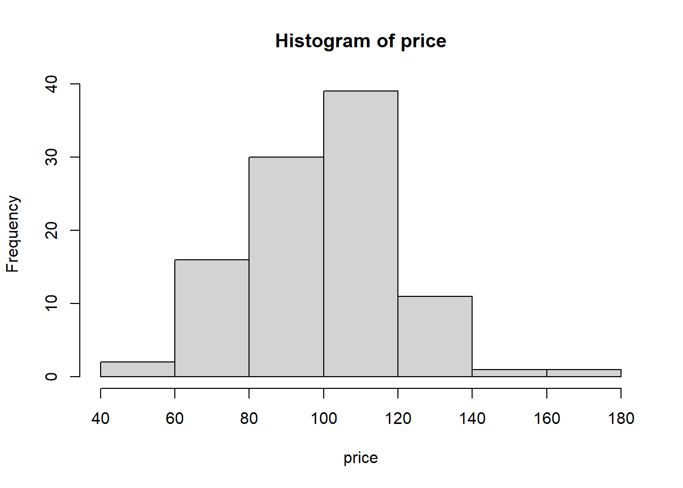
Ah, so what we see is that unsurprisingly bodyfat is strongly correlated with bmi. This gets into a key point of regression - having two variables that explain the same thing can actually hurt your model fit. Sure, bodyfat predicted healthcare costs when standing alone, but it’s correlation with bmi is what was indirectly driving that relationship. This became clear when we included both features in the same model.
While this is simple to deal with now, what happens when you have lots of features (hundreds? thousands?), many of which may be correlated with each other? Well, we’ll learn all sorts of fun methods to deal with that later in the course!
4.3.4 Qualitative predictors
It’s incredibly common to have features that are not continuous like age or bmi, but instead are discreet categories like yes/no. We have several in our dataset including smoker and sex. We can include these features alone or in combination with others. Let’s focus on just smoking for now.
4.3.4.1 Modeling just the effect of smoking
smoker_mod <- lm(charges ~ smoker, data = costs)
summary(smoker_mod)
##
## Call:
## lm(formula = charges ~ smoker, data = costs)
##
## Residuals:
## Min 1Q Median 3Q Max
## -19221 -5042 -919 3705 31720
##
## Coefficients:
## Estimate Std. Error t value Pr(>|t|)
## (Intercept) 8434.3 229.0 36.83 <2e-16 ***
## smokeryes 23616.0 506.1 46.66 <2e-16 ***
## ---
## Signif. codes: 0 '***' 0.001 '**' 0.01 '*' 0.05 '.' 0.1 ' ' 1
##
## Residual standard error: 7470 on 1336 degrees of freedom
## Multiple R-squared: 0.6198, Adjusted R-squared: 0.6195
## F-statistic: 2178 on 1 and 1336 DF, p-value: < 2.2e-16Well, smoking is clearly terrible for you. Let’s consider out model output.
Our \(RSE\) at 7470 is much smaller than even our
bmi_age_modmodel with it’s \(RSE\) of 1.1387^{4}.This lower error is reflected in our \(R^2\) which indicates that smoking alone explains 61.98% of the variation in healthcare costs. Age and BMI only explained 11.72% of the variation. So although those are important, smoking clearly has a major impact on healthcare costs.
Our \(\hat{\beta}_1\) is now just a binary effect. What that means is that smokers will (note how the coeficent is named
smokeryes) you pay an additional $2.361596^{4} on average! Why doesn’t it say what the effect of not smoking is? We’ll, when you fit binary measures R chooses one of them as a baseline and thus measures the effect relative to that.
We can make a quick figure to visualize this effect. A boxplot would work nicely as we have a categorical variable and a continuous variable.
ggplot(costs,
    aes(x = smoker, y = charges)) +
geom_boxplot() 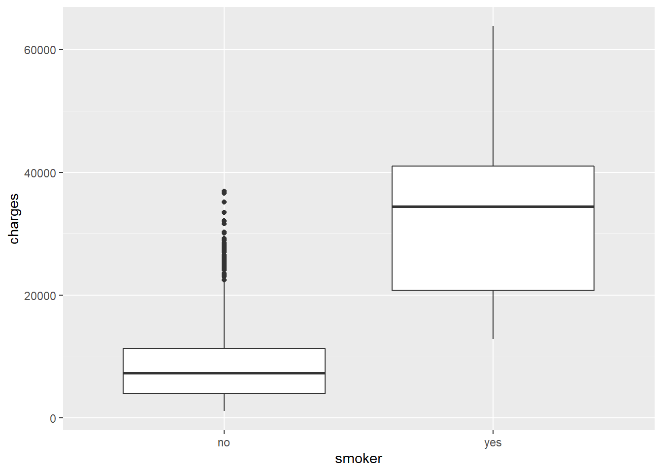
4.3.5 Interactions between features
Multiple regression models don’t have to be just the addition of multiple features. Instead, they can also have interactions among features. It might be reasonable to assume that that the effect of BMI on healthcare costs isn’t linear, but instead increases with say age. In other words, a high BMI at a young age might have a lower effect on healthcare cost while that same high BMI at an older age might have a higher healthcare cost.
Let’s fit a model looking at how and if smoking interacts with the BMI of an individual. You fit interaction terms by simply using the multiplication operator between the terms instead of the addition operator
bmi_smoker_mod <- lm(charges ~ bmi * smoker, data = costs)
summary(bmi_smoker_mod)
##
## Call:
## lm(formula = charges ~ bmi * smoker, data = costs)
##
## Residuals:
## Min 1Q Median 3Q Max
## -19768.0 -4400.7 -869.5 2957.7 31055.9
##
## Coefficients:
## Estimate Std. Error t value Pr(>|t|)
## (Intercept) 5879.42 976.87 6.019 2.27e-09 ***
## bmi 83.35 31.27 2.666 0.00778 **
## smokeryes -19066.00 2092.03 -9.114 < 2e-16 ***
## bmi:smokeryes 1389.76 66.78 20.810 < 2e-16 ***
## ---
## Signif. codes: 0 '***' 0.001 '**' 0.01 '*' 0.05 '.' 0.1 ' ' 1
##
## Residual standard error: 6161 on 1334 degrees of freedom
## Multiple R-squared: 0.7418, Adjusted R-squared: 0.7412
## F-statistic: 1277 on 3 and 1334 DF, p-value: < 2.2e-16Wow, this model is explaining 74.1771% of the variation in healthcare costs. That’s incredibly impressive. Let’s think a bit about what the interaction here is doing. If we look, we now have three parameters ( bmi, smokeryes, and bmi:smokeryes). Of course, there are three associated \(\hat{\beta}\) coefficents:
\(\hat{\beta}_1\) is for
bmi, which is the usual positive effect of body mass index on healthcare costs.\(\hat{\beta}_2\) is then the estimate for if someone is a smoker. What’s confusing is that it’s a huge negative number. Why would being a smoker reduce your healthcare costs? Well, you need to consider it alongside the interaction.
\(\hat{\beta}_3\) is now our estimate for our interaction between
bmiandsmoker. You can think of this as a ‘slope modifier’ for bmi, where the effect of bmi changes on if they’re a smoker or not. So people who are not smokers will have the slope of just \(\hat{\beta}_1\), while those that are have a slope of \(\hat{\beta}_1\) + \(\hat{\beta}_3\) and the binary addition of \(\hat{\beta}_2\)
This makes sense when you look at formulas to calculate our \(y\) for each observation: \[y_{smoker} = \hat{\beta}_1 \cdot bmi + \hat{\beta}_2 \cdot 1 + \hat{\beta}_3 \cdot bmi \cdot 1\] \[y_{non-smoker} = \hat{\beta}_1 \cdot bmi + \hat{\beta}_2 \cdot 0 + \hat{\beta}_3 \cdot bmi \cdot 0\] So why the negative \(\hat{\beta}_2\)? Well, the lowest bmi in our dataset is 15.96, so when you consider the negative \(\hat{\beta}_2\) alongside the positive \(\hat{\beta}_3\) you will still have a positive increase in healthcare costs even at the lowest bmi. This gets to the big issue with interaction plots. They’re really tricky to interpret from coefficients alone, especially when your interaction is between two continuous variables rather than just one. Let’s take some time to plot this model:
4.3.6 Plotting interaction terms
This will be a touch complicated, but if you can figure this out then any simpler plot will be cake. Let’s think about our question and what we’re trying to plot. First we have a continuous target and one continuous feature. Normally when you have two continuous datatypes you’re trying to plot you use a scatterplot. Second we also have our binary effect of smoking. The best way to do this is to plot two lines, one for each formula above!
How do we do this? ggplot will plot a simple line if you just give it a vector of \(x\) and \(x\) values. Given \(y\) is a function of \(x\), we will need one \(x\) vector and then calculate two \(y\) vectors (one for smokers and one for non-smokers - just use each formula).
Our \(x\) vector is just a range of bmi values present in the data. It must be equal to the length of our dataset otherwise ggplot gets unhappy.
costs_n <- nrow(costs) #nrow() gets the number of rows in a dataframe

# The function seq() generates sequences in a range of values
# You provide the starting value of the sequence
# Then the max value
# Then how long you want the resulting sequence to be - in this case the length of the data frame
bmi_seq <- seq(min(costs$bmi), max(costs$bmi), length.out = costs_n)
Now we need to punch this range of \(x\) values into our formulas. How do we easily get our model coefficients? We store the summary to an object and then can access all sorts of values from the summary using the $ operator. Watch:
int_model <- summary(bmi_smoker_mod) #store model summary
int_model$coefficients # use $ to access data within
## Estimate Std. Error t value Pr(>|t|)
## (Intercept) 5879.42472 976.86903 6.018642 2.269276e-09
## bmi 83.35055 31.26854 2.665636 7.777063e-03
## smokeryes -19066.00272 2092.02814 -9.113645 2.841138e-19
## bmi:smokeryes 1389.75576 66.78297 20.810032 1.608349e-83We can now use data frame slicing to get our \(\hat{\beta}\) coefficients. For example:
int_model$coefficients[2,1] #beta_1 via slicing## [1] 83.35055Let’s now just calculate our two \(y\) vectors
y_smoker <- int_model$coefficients[1,1] + int_model$coefficients[2,1] * bmi_seq +
  int_model$coefficients[3,1] * 1 +
  int_model$coefficients[4,1] * bmi_seq * 1

# Same formula but just use zeros as they are not smokers and thus the value is 0
y_nonsmoker <- int_model$coefficients[1,1] + int_model$coefficients[2,1] * bmi_seq + int_model$coefficients[3,1] * 0 + int_model$coefficients[4,1] * bmi_seq * 0
And now we can plot! This will be more complex as we’re need to do three things on one plot:
1. Make a scatterplot with the original data
2. Make a line using bmi_seq for the \(x\) and y_smoker for the \(y\)
3. Make a line using bmi_seq for the \(x\) and y_nonsmoker for the \(y\)
Let’s just make the scatter to start!
ggplot(costs,
    aes(x = bmi, y = charges)) +
 geom_point()
Let’s now add on a geom_line() for our first line. It will have its own aesthetic as follows:
ggplot(costs,
    aes(x = bmi, y = charges)) +
 geom_point() +
 geom_line(aes(x = bmi_seq, y = y_smoker))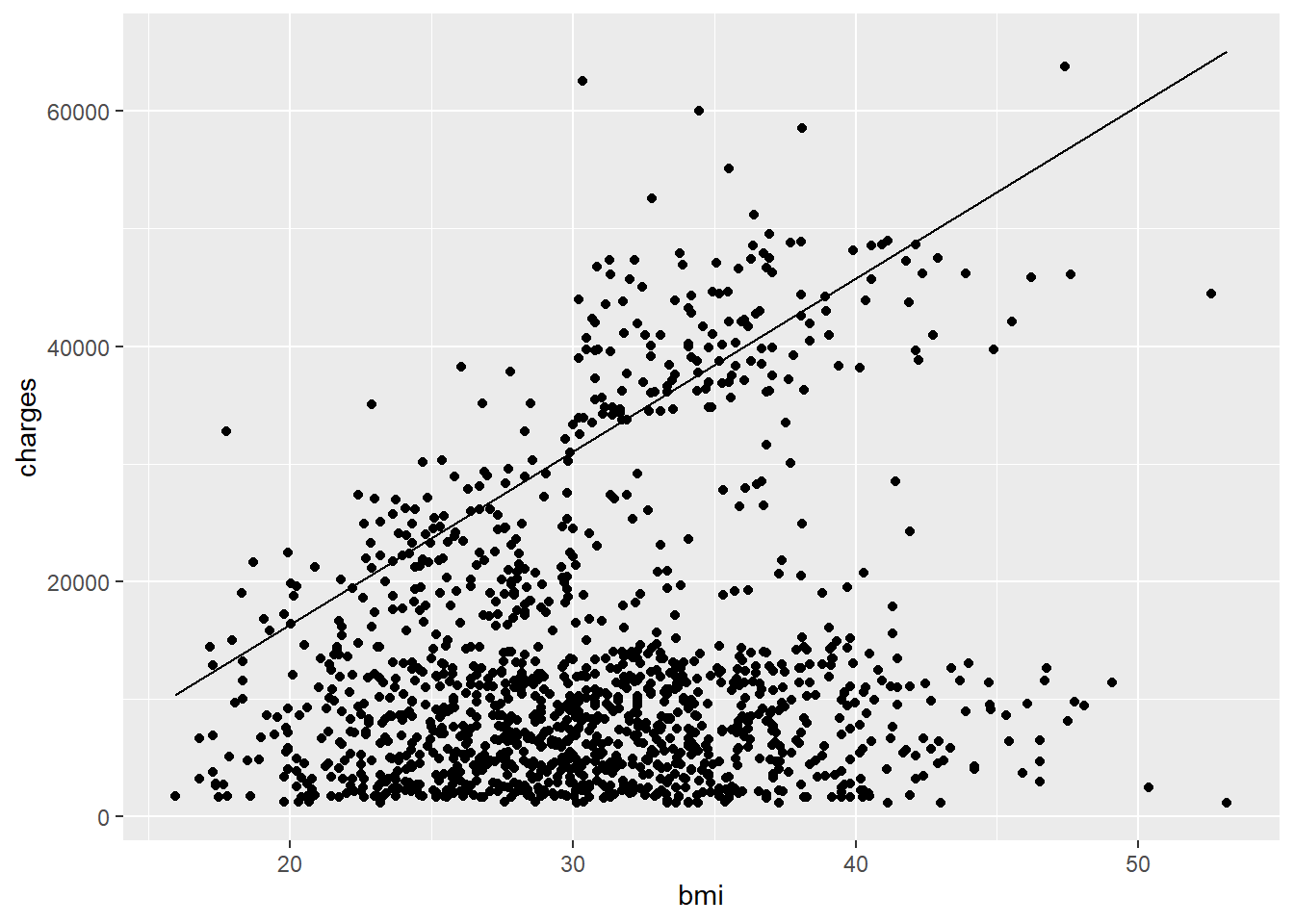
Now the second line. Also add color = smoker to an aes() argument inside geom_point() and see what it does.
ggplot(costs,
    aes(x = bmi, y = charges)) +
 geom_point(aes(color = smoker)) +
 geom_line(aes(x = bmi_seq, y = y_smoker)) +
 geom_line(aes(x = bmi_seq, y = y_nonsmoker))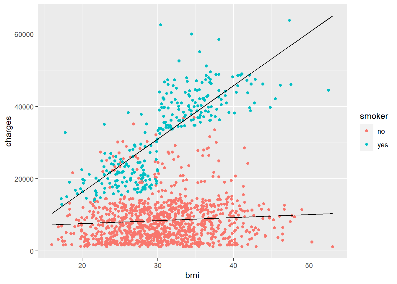
Wow. So clearly smoking has a major effect on healthcare costs! What’s interesting is that the lines still don’t fit perfectly, suggesting there’s other factors at play. Maybe some additional interactions and/or features would help. We’ll stop here for now, but hopefully you’ve gotten a good idea how to fit and interpret more than a basic regression model.