12 Regularization
Up to this point we’ve been fitting various types of models (linear regression, logistic regression, kNN) to predict some continuous or categorical target. We’ve been working with pretty simple datasets that don’t have an overly massive number of features and have a good number of observations. Together this makes it easy to fit and interpret the models.
But, in the age of big data we often have a massive number of features. It’s so easy to collect so many details… if you’re Netflix you will be taking in every user’s age, gender, income, length of watching a TV show, last show watched, number of action shows watched, number of romantic comedies watched, time of day last watched, number of times a week watched, how long you hovered over something, and hundreds of other things. In this case, how do we know which ones to use? Should we just include them all? That isn’t a good solution as the more features you include the more flexible your model is and thus you may start seeing high variance and thus high test error. Even if it doesn’t have high test error, what if you have 50 features that are significant… how do you interpret which ones are the most important? Other times we may have lots of features but relatively few rows of data. What do we do in this case?
Chapter 6 of your book deals solely with this issue. How do we fit and find the optimal model when there are thousands or million potential combinations of features, each of which would need to be fit with itss own model? We’re going to cover model regularization in detail, but I want to briefly cover the other methods here even though we’re not going to actually apply them beyond this.
12.1 Dealing with lots of features - a few methods in brief
Let’s use the Olympic dataset that’s part of the ade4 package. This is a dataset where you can try and predict the score in an Olympic decathlon based on performance in the 10 events. There are only 33 observations, but then the 10 features, which makes this ideal for illustrating how having lots of features can be a problem as it’s so easy to overfit.
library(ade4)Load data, convert to a data frame, check it out. We see that we have the 10 different events and then a score feature
data("olympic")
oly <- data.frame(olympic)
glimpse(oly)
## Rows: 33
## Columns: 11
## $ tab.100 <dbl> 11.25, 10.87, 11.18, 10.62, 11.02, 10.83, 11.18, 11.05, 11...
## $ tab.long <dbl> 7.43, 7.45, 7.44, 7.38, 7.43, 7.72, 7.05, 6.95, 7.12, 7.28...
## $ tab.poid <dbl> 15.48, 14.97, 14.20, 15.02, 12.92, 13.58, 14.12, 15.34, 14...
## $ tab.haut <dbl> 2.27, 1.97, 1.97, 2.03, 1.97, 2.12, 2.06, 2.00, 2.03, 1.97...
## $ tab.400 <dbl> 48.90, 47.71, 48.29, 49.06, 47.44, 48.34, 49.34, 48.21, 49...
## $ tab.110 <dbl> 15.13, 14.46, 14.81, 14.72, 14.40, 14.18, 14.39, 14.36, 14...
## $ tab.disq <dbl> 49.28, 44.36, 43.66, 44.80, 41.20, 43.06, 41.68, 41.32, 42...
## $ tab.perc <dbl> 4.7, 5.1, 5.2, 4.9, 5.2, 4.9, 5.7, 4.8, 4.9, 5.2, 4.8, 4.7...
## $ tab.jave <dbl> 61.32, 61.76, 64.16, 64.04, 57.46, 52.18, 61.60, 63.00, 66...
## $ tab.1500 <dbl> 268.95, 273.02, 263.20, 285.11, 256.64, 274.07, 291.20, 26...
## $ score <dbl> 8488, 8399, 8328, 8306, 8286, 8272, 8216, 8189, 8180, 8167...12.1.1 Subset selection
One method of reducing the number of features involves fitting models and then adding/removing features based on if they improve fit. You could fit all possible model combinations, but this will rapidly explode into fitting thousands or more models. Other simpler methods involved adding (forwards stepwise selection) or removing features (backwards stepwise selection) based on if they improve fit. These forward and backward methods which are conceptually similar. Thinking about forward, we’d start by fitting the following model.
lm(score ~ tab.100, data = oly)
Then we’d add another feature. If it improves the R2 (or some other model fit measure of choice) then we’d keep that extra feature. Say this model.
lm(score ~ tab.100 + tab.long, data = oly)
Great, we can say that helped, so let’s add another feature.
lm(score ~ tab.100 + tab.long + tab.poid, data = oly)
Let’s say that tab.poid didn’t help, then we remove it and replace with something else.
lm(score ~ tab.100 + tab.long + tab.haut, data = oly)
While this in theory is less computationally intensive as just fitting all possible models, it’s also clunky and doesn’t guarantee that you wound up with the best model. This is because as we’ve seen in earlier chapters the relative importance of one feature can depend on the inclusion of another. Thus, the order in which features are added and removed will influence what model you wind up with. You might have found a different best model if you started down a different “path” by fitting a different feature first. Finally, there is debate out there if repeatedly fitting different combinations isn’t what’s called multiple hypothesis testing. The problem that arises when you fit models in such a non-specific way repeatedly to the same dataset is that you can stumble upon significant p-values (indeed, using a p = 0.05 threshold we’d expect to see something significantly non zero 5% of the time even when it’s not a true effect).
Point being, although it is a method that’s out there, it for sure has its own set of issues that you should be aware of!
12.1.2 Penalizing models for having too many features
12.1.2.1 Adjusted \(R^2\)
Another way to ensure you don’t have too many features in your model is to fit say some subset of models, but then use a fit metric that adds a penalty for each extra parameter.
We remember our \(R^2\) measure which is calculated from your total sum of squares (\(TSS\)) and the residual sum of squares (\(RSS\)) of the fitted model \[R^2 = 1 - \frac{RSS}{TSS}\]
Well there’s also an Adjusted \(R^2\) measure which penalizes based on the number of features, \(d\). You can see from the formula below that the numerator with the \(RSS\) will shrink as more parameters and included. Thus, your adjusted \(R^2\) will be smaller than a non-adjusted \(R^2\) \[Adjusted\:R^2 = 1 - \frac{RSS/(1-n-d)}{TSS/(1-n)}\]
12.1.2.2 AIC, BIC, DIC, Cp
AIC, BIC, and DIC are other commonly used methods to penalize your model’s fit based on number of features. These are all scores that you calculate when fitting different models, and then compare the models using the score. The best model is then the one with the lowest score. These methods are very commonly used in academia (I’ve published lots of papers using them), but less-so for non-academic purposes.
The AIC formula is below (and the others are very similar and thus just refer to your book). The key thing to notice is that AIC will grow for every additional parameter. Thus, given you judge fit based on which models have the lowest AIC, models with an extra parameter must have a much lower RSS (and thus much better fit) in order to offset the extra parameter penalty. \[AIC = \frac{1}{n\hat\sigma^2}(RSS + 2d\hat\sigma)\]
12.2 Shrinkage methods - AKA Regularization
The class of models that we’re going to focus on use what’s called regularization. Remember that when fitting a linear regression model the goal is to find the fit line that has the smallest residual sum of squares \(RSS\)?
The closer the estimated y value is (\(\hat{y}\)) is to the actual value of \(y\), the lower the \(RSS\). You can minimize this value using the formulas to calculate \(\beta_1\) and \(\beta_0\) that we learned back in our linear regression lesson. The point here is that the goal is to minimize \(RSS\) \[\sum_{x = 1}^{n} (\hat{y}_i - y_i)^2 = RSS\] Well, what regularization does is make is so you instead minimize \(RSS\) PLUS another value that gets bigger as your \(\beta\) estimates grow. This biases the model in favor of using smaller, more conservative \(\beta\) coefficients, which will likely have lower variance than the non-regularized regression models.
The two models we’re going to learn about are Ridge Regression and Lasso Regression. These both rely on this concept of shrinking your \(\beta\) coefficients through a penalty. This shrinking allows you to fit all your features without the worries of overfitting, and thus having high variance and poor test error, or having to do some sort of stepwise selection.
Let’s start with Ridge Regression
12.2.1 Ridge Regression
Ridge regression fits a regression model by minimizing the following. The \(RSS\) is the same, but you now have to minimize the right part of the equation as well. The \(\sum_{j=1}^{p}\beta_{j}^2\) is saying that part of what it’s trying to minimize is the sum of your squared \(\beta\) coefficients. Thus it’ll try to shrink or minimize your \(\beta\)’s as part of fitting the model. The other key part is the \(\lambda\) (lambda). \(\lambda\) is what’s known as a tuning parameter or hyperparameter. I’ll get to how we find our optimal \(\lambda\) next, but for now the key thing to realize is that if we put in a small lambda, the model won’t be penalized for large \(\beta\)’s, and thus won’t shrink them that much. Indeed, if it’s zero then it’s just regular old least squares regression! But, as \(\lambda\) grows the model will start penalizing your \(\beta\)’s more and more and thus will shrink your coefficients towards zero! This is pretty cool as what it’s letting you do is fit all your features, but making all the features with little importance have little to no effect (or removing them entirely).
\[RSS + \lambda\sum_{j=1}^{p}\beta_{j}^2\] #### A quick note on \(\lambda\) before fitting
As mentioned above, how do we find the optimal \(\lambda\) value for our model? Too small and we won’t penalize enough and thus get high variance in our test data, too large and we’ll penalize too much and get high bias in our test data. Both result in high test error, which is bad. The ideal way to tackle this would be to test a range of \(\lambda\) values and see which one gives the lowest error. Thus we are ‘tuning’ the parameter to find it’s ideal value. Luckily the package we’re going to use can not only take a range of \(\lambda\) values, but it’ll cross-validate them as well all in one go!
12.2.1.1 Fitting our Ridge Regression model
Let’s use the Olympic decathlon data for this example. We’re going to start by splitting our data, then finding our optimal \(\lambda\), then using that \(\lambda\) value to fit our model. We’ll be using the package glmnet which we’ll load now.
library(glmnet)12.2.1.1.1 Splitting our data
Although glmnet is great at fitting models, it doesn’t allow you to specify your models in the target ~ features syntax that we’re used to. Instead you need your features (x) to be a matrix. We can use the function model.matrix() to convert our data frame to a matrix of features. The nice part is this will also one hot encode any categorical variables for you.
Below we use the model.matrix() function, feeding it the formula of “target ~ .” so the model knows what is the target and what isn’t. You also specify where to find the data, of course. The [,-1] is removing the intercept that the function will calculate. Check the book for why we don’t need this. We also just grab our target value score and assign it to target.
set.seed(888) # set seed for reproducibility

features <- model.matrix(score~., data = oly)[,-1] # convert features to matrix
target <- oly$score # get target

split_index <- createDataPartition(oly$score, p = 0.7, list = F) # create split_index

#split data as usual.
#Note we don't need to select column for features as we already removed the target!
features_train_m <- features[split_index,]
features_test_m <- features[-split_index,]
target_train_m <- target[split_index]
target_test_m <- target[-split_index]
12.2.1.2 Finding \(\lambda\)
Let’s find our \(\lambda\) now. First we’ll specify a exponential sequence that ranges from tiny (0.01) to huge (10^10). We do this by making a sequence from -2 to 10 with 100 values in between and then taking 10^each value in the sequence. Go play with the individual code directly in the console to better understand how this is done. For example, go enter seq(-2, 10, length = 100). For now, we’ll just generate our vector of lambda values.
lambda_vals <- 10^seq(-2, 10, length = 1000)
lambda_vals[c(1,2,3, 998,999,1000)] # look at first and last three to check
## [1] 1.000000e-02 1.028045e-02 1.056876e-02 9.461848e+09 9.727203e+09
## [6] 1.000000e+10Now we’ll use the cv.glmnet() function to fit our model across the varying lambdas. We specify our features first, then target. the alpha = 0 is telling glmnet() that you want this to be ridge regression (alpha = 1 is for LASSO). We can then call the lambda.min from our model object to give us the \(\lambda\) value that has the lowest \(MSE\). We can ignore the warning.
ridge_cv <- cv.glmnet(features_train_m, target_train_m, alpha = 0, lambda = lambda_vals, grouped = FALSE)
bestlam <- ridge_cv$lambda.min
bestlam # value of lambda that minimizes error
## [1] 2.9004312.2.1.3 Using our optimal lambda to fit the model and generate predictions
Let’s use that \(\lambda\) to fit our model and make predictions. We’ll first specify a general model with just glmnet(), then use our trusty predict() function to generate target predictions using our test features. We can tell it what \(\lambda\) to use when we specify s. One thing that differs here is that we don’t tell it our test features using newdata =. Instead we use newx =.
# fit model
ridge_mod <- glmnet(features_train_m, target_train_m, alpha = 0)

# get predictions
ridge_preds <- predict(ridge_mod, s = bestlam, newx = features_test_m)

# calculate MSE
mean((ridge_preds - target_test_m)^2)
## [1] 4900.913And there we have the test \(MSE\) of our ridge regression model! In order to know if this is good or bad we’ll want to cross validate it and compare to other models, which we’ll get to later.
12.2.1.4 Exploring our \(\beta\) coefficients and the effect of \(\lambda\)
Let’s take a minute to show how our \(\lambda\) value influences shrinkage of our \(\beta\)’s.
First, to get our coefficients from a glmnet() model we need to use predict() with some slight modification. We can see how performance in each event influences overall score in the decathlon. tab.100 is for time in the 100m dash. It’s not surprising that for every extra second it takes one to complete that their score drops by -247.75 points. For every extra meter someone throws a javelin, we see an increase in score by 15.15 points.
ridge_coef <- predict(ridge_mod, type = "coefficients", s = bestlam)[1:11,]
ridge_coef
## (Intercept) tab.100 tab.long tab.poid tab.haut tab.400
## 8892.77251 -247.74824 227.14713 59.12515 897.85635 -47.26363
## tab.110 tab.disq tab.perc tab.jave tab.1500
## -108.95045 18.07661 288.76504 15.15348 -5.63988Let’s show what happens when we increase our \(\lambda\). Currently our lambda is
bestlam## [1] 2.90043This is really small and suggests that with the current split we are not having to regularize very much. We can rerun the above but instead specify a larger \(\lambda\) in the s = argument. Notice how a lot of our \(\beta\) coefficients shrink closer to zero when \(\lambda\) = 100. That is forcing them to have less importance.
ridge_coef <- predict(ridge_mod, type = "coefficients", s = 100)[1:11,]
ridge_coef
## (Intercept) tab.100 tab.long tab.poid tab.haut tab.400
## 8936.540199 -237.586430 223.727287 64.995875 841.785737 -48.036237
## tab.110 tab.disq tab.perc tab.jave tab.1500
## -105.975171 15.066914 257.297538 13.366074 -4.663467Let’s try a huge \(\lambda\). We see that most of our \(\beta\)’s are near zero now.
ridge_coef <- predict(ridge_mod, type = "coefficients", s = 1000000)[1:11,]
ridge_coef
## (Intercept) tab.100 tab.long tab.poid tab.haut
## 7.855720e+03 -9.931595e-34 8.884643e-34 2.375378e-34 2.525939e-33
## tab.400 tab.110 tab.disq tab.perc tab.jave
## -1.960888e-34 -5.001708e-34 4.291940e-35 8.180136e-34 3.534778e-35
## tab.1500
## -9.505518e-36What about when \(\lambda\) = 0?
ridge_coef <- predict(ridge_mod, type = "coefficients", s = 0)[1:11,]
ridge_coef
## (Intercept) tab.100 tab.long tab.poid tab.haut tab.400
## 8892.77251 -247.74824 227.14713 59.12515 897.85635 -47.26363
## tab.110 tab.disq tab.perc tab.jave tab.1500
## -108.95045 18.07661 288.76504 15.15348 -5.63988Those are virtually identical to a regular multiple regression model! So, the smaller the \(\lambda\) the lower the shrinkage, while the bigger the \(\lambda\) the greater the shrinkage.
#bind training data back together
oly_full <- data.frame(features_train_m, target_train_m)
oly_full <- oly_full %>% rename(score = 'target_train_m') # rename
lr_mod <- lm(score ~ ., data = oly_full) # fit
summary(lr_mod)$coefficients[,1] # get beta coefficients
## (Intercept) tab.100 tab.long tab.poid tab.haut tab.400
## 8863.518740 -252.615719 227.809833 47.257327 905.330092 -43.096275
## tab.110 tab.disq tab.perc tab.jave tab.1500
## -115.480683 21.511068 312.386062 16.551194 -6.41797512.2.2 Lasso Regression
Lasso works much like ridge regression. It still uses \(\lambda\) in the same way, but it differs in how it penalizes based on \(\beta\) coefficients. Instead of using \(\lambda\sum_{j=1}^{p}\beta_{j}^2\) it uses \(\lambda\sum_{j=1}^{p}|\beta_{j}|\). Because of this it allows the model to actually push coefficient to zero, thus selecting features for you. Be sure to read about how this is done in the book itself.
Let’s fit our Lasso model
12.2.2.1 Finding \(\lambda\)… again
We need to find the optimal \(\lambda\) again. We’ll use the same process as before. The only change now is that to fit a lasso model we specify alpha = 1 in our cv.glmnet() function.
lambda_vals <- 10^seq(-2, 10, length = 1000)
lambda_vals[c(1,2,3, 998,999,1000)] # look at first and last three to check
## [1] 1.000000e-02 1.028045e-02 1.056876e-02 9.461848e+09 9.727203e+09
## [6] 1.000000e+10lasso_cv <- cv.glmnet(features_train_m, target_train_m, alpha = 1, lambda = lambda_vals, grouped = FALSE)
bestlam <- lasso_cv$lambda.min
bestlam # value of lambda that minimizes error## [1] 0.0112.2.2.2 Calculating MSE of our Lasso model
Following the same fitting procedure as before. Here are Lasso model appears to be doing better than our ridge model, but given the data is so small we want to cross validate these results a bunch of times. We’ll do that a bit later.
# fit model
lasso_mod <- glmnet(features_train_m, target_train_m, alpha = 1)

# get predictions with cross validated lambda
lasso_preds <- predict(lasso_mod, s = bestlam, newx = features_test_m)

# calculate MSE
mean((lasso_preds - target_test_m)^2)
## [1] 4804.73312.2.2.3 Playing with \(\lambda\)
Just to illustrate how our Lasso model will actually zero out coefficients, let’s input a \(\lambda\) of 200. Doing so we see that most of our \(\beta\) coefficients are now zero. This means the model doesn’t even try and predict with unimportant features.
lasso_coef <- predict(lasso_mod, type = "coefficients", s = 200)[1:11,]
lasso_coef
## (Intercept) tab.100 tab.long tab.poid tab.haut tab.400
## 5586.54641 0.00000 217.23221 27.57721 0.00000 0.00000
## tab.110 tab.disq tab.perc tab.jave tab.1500
## 0.00000 0.00000 70.27826 0.00000 0.0000012.2.3 Cross-validating our models
Of course, we learned last week that we should calculate an average test error for our models as randomness in the splits can cause variation in test error. Thus, by looking at many splits you gain more confidence in the accuracy of your models.
12.2.4 Making our split and empty data frame
First, we’ll make our split index but set times = to 100 so we generate 100 split indexes. We’re doing 100 folds given the sample size is so small we will likely have lots of variation of error across samples. Doing more folds helps us hone in on a more stable measure.
split_index <- createDataPartition(oly$score, p = 0.7, list = F, times = 100)Now we’ll make our empty data frame
comp_df <- data.frame(matrix(ncol = 4, nrow = ncol(split_index)))
colnames(comp_df) <- c('lin_reg_mse', 'ridge_mse', 'lasso_mse' ,'fold')
12.2.4.1 Making our for loop
Below is a loop that splits our data, runs a model, and fills our empty data frame with the errors. You’ll notice that I also include code to fit a regular linear regression model in there so we can see if this regularization is helping over that.
for(i in 1:ncol(split_index)) {
 # split for linear regression
 features_train <- oly[split_index[,i], !(colnames(oly) %in% c('score'))]
 features_test <- oly[-split_index[,i], !(colnames(oly) %in% c('score'))]
 target_train <- oly[split_index[,i], c('score')]
 target_test <- oly[-split_index[,i], c('score')]
 # preprocess for linear regression
 oly_pp <- preProcess(features_train, method = c('scale'))
 features_train <- predict(oly_pp, newdata = features_train)
 features_test <- predict(oly_pp, newdata = features_test)
 # join and rename features and target
 training <- data.frame(features_train, target_train)
 training <- training %>%
  rename(score = target_train)
 # fit linear regression
 reg_mod <- lm(score ~ ., data = training)
 reg_pred <- predict(reg_mod, newdata = features_test)
 # calculate MSE and add to DF
 reg_mse <- mean((target_test - reg_pred)^2)
 comp_df[i, 'lin_reg_mse'] <- reg_mse
 comp_df[i, 'fold'] <- i
 # generate x and y (this doesn't have to be here but will leave for clarity)
 features <- model.matrix(score~., oly)[,-1]
 target <- oly$score
 lambda <- 10^seq(10, -2, length = 100)
 # split x and y
 features_train_m <- features[split_index[,i],]
 features_test_m <- features[-split_index[,i],]
 target_train_m <- target[split_index[,i]]
 target_test_m <- target[-split_index[,i]]
 # fit ridge model
 ridge_mod <- glmnet(features_train_m, target_train_m, alpha = 0)
 cv_out <- cv.glmnet(features_train_m, target_train_m, alpha = 0, lambda = lambda, grouped = FALSE)
 bestlam <- cv_out$lambda.min
 ridge_pred <- predict(ridge_mod, s = bestlam, newx = features_test_m)
 # calculate error and add
 ridge_mse <- mean((target_test_m - ridge_pred)^2)
 comp_df[i, 'ridge_mse'] <- ridge_mse
 # same for lasso
 lasso_mod <- glmnet(features_train_m, target_train_m, alpha = 1)
 cv_out <- cv.glmnet(features_train_m, target_train_m, alpha = 1, lambda = lambda, grouped = FALSE)
 bestlam <- cv_out$lambda.min
 lasso_pred <- predict(lasso_mod, s = bestlam, newx = features_test_m)
 lasso_mse <- mean((lasso_pred - target_test_m)^2)
 comp_df[i, 'lasso_mse'] <- lasso_mse

}
12.2.4.2 graphing our results
Let’s do some data wrangling to make our data in a easier to read format for ggplot
Currently the format is ‘wide’ such that each error measure type has it’s own column.
head(comp_df)## lin_reg_mse ridge_mse lasso_mse fold
## 1 431.4795 876.8839 463.8869 1
## 2 343.0930 334.8495 307.8185 2
## 3 312.6817 654.1425 329.3818 3
## 4 1269.7818 1316.6070 1198.3101 4
## 5 5798.1215 4533.6053 5572.5744 5
## 6 3698.2821 4470.8438 4494.1759 6But really most languages work better if the data is in ‘long’ format such that error type is its own factor with it’s associated measure. We can use the gather() function that’s part of tidyverse to ‘gather’ our columns into a single one.
data_long <- gather(data = comp_df, key = type, value = error, c('lin_reg_mse', 'ridge_mse', 'lasso_mse' ), factor_key=TRUE)
data_long[c(1,2,3,101,102,103,201,202,203),]# check out a few values
## fold type error
## 1 1 lin_reg_mse 431.4795
## 2 2 lin_reg_mse 343.0930
## 3 3 lin_reg_mse 312.6817
## 101 1 ridge_mse 876.8839
## 102 2 ridge_mse 334.8495
## 103 3 ridge_mse 654.1425
## 201 1 lasso_mse 463.8869
## 202 2 lasso_mse 307.8185
## 203 3 lasso_mse 329.3818This is a better format as we can plot different lines by color by just specifying color = type inside our aesthetic call.
ggplot(data_long,
    aes(x = fold, y = error, color = type)) +
 geom_line() +
 labs(x = 'Fold Number', y = 'Mean Squared Error') +
 theme_classic()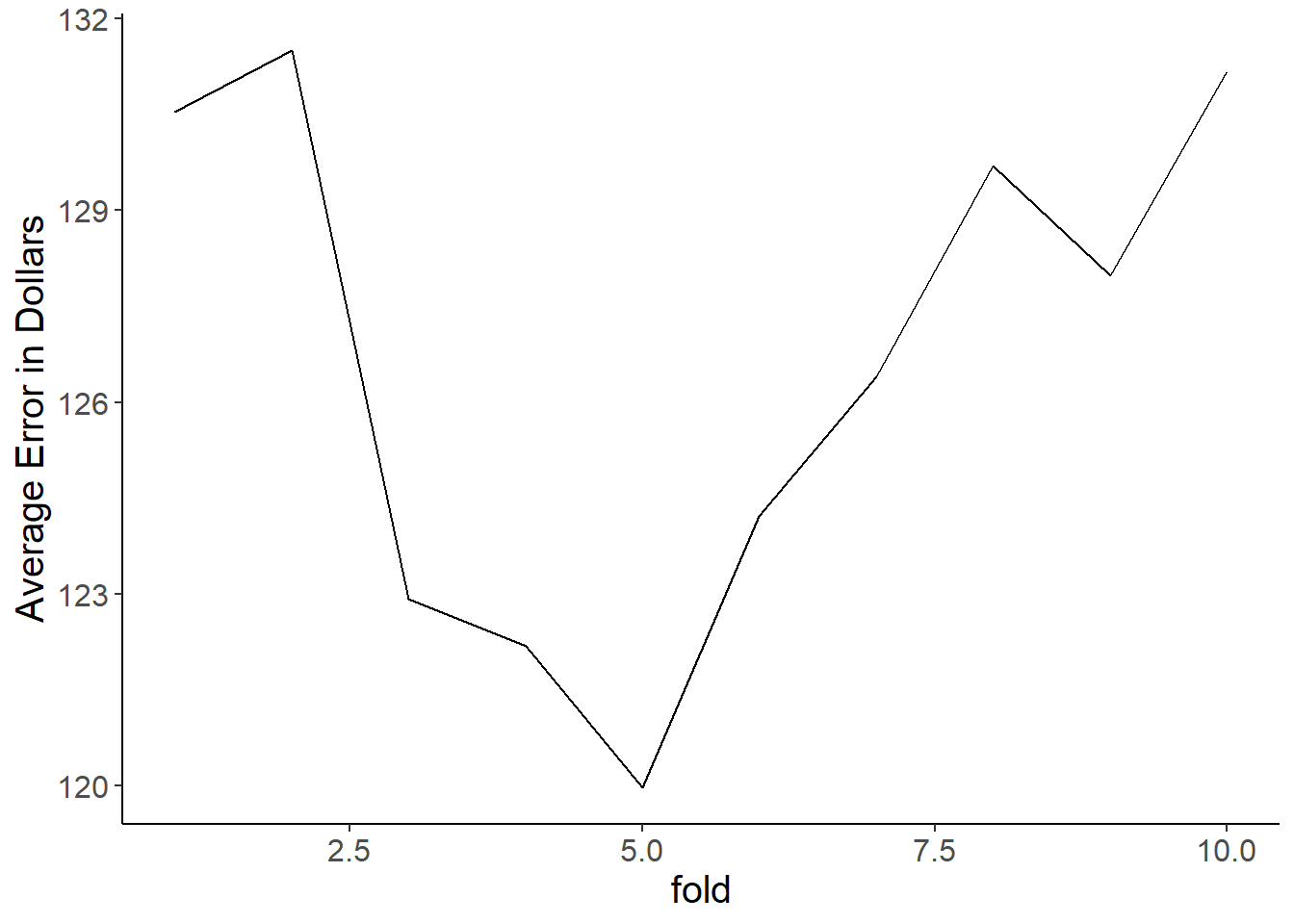
And let’s take the mean \(MSE\) of each model while we’re at it.
mean(comp_df$lin_reg_mse)## [1] 3031.229mean(comp_df$ridge_mse)## [1] 2893.818mean(comp_df$lasso_mse)## [1] 3130.283Looks like our ridge did the best. Let’s see what the actual mean error in our predictions is by taking the square root of the mean square error.
sqrt(mean(comp_df$ridge_mse))## [1] 53.7942212.2.4.3 Interpreting our figure and wrapping up.
So, it looks like our ridge regression generally performs the best. This is clear given it has the lowest average \(MSE\) over our 100 folds. On average we can see that our score predictions are off by 54 points when using ridge regression. We can see from the graph that the \(MSE\) estimates for all models jump around a ton. This shouldn’t surprise us given we have only 33 observations total and thus our test set is only 8 values with the current split proportion! It is all too easy both overfit a model with such limited training data and get really strange test sets that are really hard to predict. Both of these will cause test \(MSE\) to jump around fold-to-fold.
Although this is a case where ridge regression is able to improve on our run of the mill least squares linear regression, that might not always be the case. In other data sets you might find that Lasso models fit better. You book covers more detail regarding situations where one might be better than the other. From this lesson you should more understand how to fit these models and what the goals of the model types are.
It’s worth wrapping up by saying that just because these models have a number of benefits over regular least squares linear regression, it doesn’t mean you should default to them. One downside is that there are extra steps of finding lambda. The bigger downside in my opinion is that although you get \(\beta\) coefficients, you don’t readily get their confidence intervals and p-values. If your goal is to make inference regarding what features explained a pattern, rather than predict new data points, then these regularization methods might not be the best. So, all these models are just tools, each of which has their own pros and cons. By learning these pros and cons you’ll be able to flexibly gain the best inference/predictive ability from a dataset rather than blindly following a cookbook.