6 Preprocessing
Preprocessing your data is far and away one of the most critical steps to any data mining pipeline. In an academic learning environment you’re often given datasets that are free of errors and have all the variables you need scaled and ready to go. In reality data are rarely this way. Most data scientists will tell you that 80% of their work is the various preprocessing steps.
What is preprocessing exactly? I’d say it can be lumped into the following general tasks:
identifying and correcting erroneous values
removing special characters and converting datatypes
filtering data to contain only the values of interest
transforming data to ensure your model runs correctly
encoding categorical variables
creating useful features
I want to stress that there isn’t a strict formula for this process… it requires you to explore your data, fix things, explore again, fix things, and so on. Every dataset is different and thus will require different combinations of techniques. Thus, the goal of this lesson is to expose you to some of these techniques and the ideas behind them, not necessarily provide a rigid structure for you to do this.
6.1 About our AirBnB data
This lesson is going to work with real data from AirBnB. They actually provide detailed listing information on their website. The raw data contained over 100 columns, but we’re only going to work with 19. The goal will be to prepare our features so that we can predict two targets within the data - rental price and rental rating. With that being said, let’s jump in!
6.2 Digging into preprocessing
6.2.1 Importing our data
Let’s load up our packages
library(tidyverse)Bring in our data
air <- read_csv("https://docs.google.com/spreadsheets/d/1q2RkNoLxyminnnUwBxqhII8bZM1OfeDXsNCGbHZW_kc/gviz/tq?tqx=out:csv")## Parsed with column specification:
## cols(
## .default = col_character(),
## minimum_nights = col_double(),
## maximum_nights = col_double(),
## square_feet = col_double(),
## bedrooms = col_double(),
## bathrooms = col_double(),
## accommodates = col_double(),
## host_identity_verified = col_logical(),
## host_is_superhost = col_logical(),
## review_scores_rating = col_double(),
## number_of_reviews = col_double()
## )## See spec(...) for full column specifications.6.3 Exploring the data set as a whole
A quick glimpse() of our data shows a bunch of columns. Right off the bat I see the following:
I see our two features that we want to use later:
priceandnumber_of_reviews.Notice how
price,cleaning_fee, andsecurity_depositare character strings because they have a $ sign in the data… we’ll have to remove those and convert to numeric before we can use the actual values within! Same with the % inhost_response_timeI see a bunch of character columns (e.g.
bed_type) that we need to look at individually and see what values are in there. We will also need to remove spaces from withinNAvalues that we need to explore
glimpse(air)## Rows: 30,218
## Columns: 21
## $ price <chr> "$50.00", "$117.00", "$80.00", "$150.00", "$...
## $ cleaning_fee <chr> "$15.00", "$35.00", "$0.00", "$95.00", "$50....
## $ security_deposit <chr> "$0.00", "$0.00", "$0.00", NA, "$200.00", "$...
## $ cancellation_policy <chr> "strict_14_with_grace_period", "moderate", "...
## $ minimum_nights <dbl> 2, 2, 2, 4, 2, 4, 2, 89, 32, 1, 32, 2, 3, 3,...
## $ maximum_nights <dbl> 89, 60, 60, 60, 365, 120, 7, 1000, 395, 730,...
## $ square_feet <dbl> NA, NA, NA, NA, NA, NA, NA, NA, NA, 1000, NA...
## $ bedrooms <dbl> 1, 3, 1, 1, 1, 2, 1, 2, 0, 2, 2, 3, 1, 1, 2,...
## $ bathrooms <dbl> 1.0, 1.0, 1.0, 1.0, 1.0, 1.0, 1.0, 2.0, 1.0,...
## $ accommodates <dbl> 1, 7, 2, 4, 2, 4, 2, 4, 3, 7, 6, 6, 2, 2, 6,...
## $ bed_type <chr> "Real Bed", "Real Bed", "Futon", "Real Bed",...
## $ room_type <chr> "Private room", "Entire home/apt", "Entire h...
## $ property_type <chr> "Condominium", "Apartment", "Apartment", "Ap...
## $ city <chr> "Chicago", "Chicago", "Chicago", "Chicago", ...
## $ neighbourhood_cleansed <chr> "Hyde Park", "South Lawndale", "West Town", ...
## $ host_identity_verified <lgl> TRUE, TRUE, FALSE, TRUE, TRUE, TRUE, TRUE, T...
## $ host_is_superhost <lgl> TRUE, TRUE, FALSE, FALSE, FALSE, FALSE, FALS...
## $ host_response_time <chr> "within an hour", "within an hour", "within ...
## $ host_response_rate <chr> "100%", "100%", "100%", "89%", "93%", "89%",...
## $ review_scores_rating <dbl> 100, 96, 92, 92, 85, 89, 100, 93, 85, 86, 86...
## $ number_of_reviews <dbl> 149, 368, 338, 35, 38, 9, 4, 9, 37, 178, 44,...Let’s look at a summary() to understand our numeric data better. Doing this the following jumps out at me:
We are missing over 4000
review_scores_ratingsand much less frombedroomsandbathrooms. We can probably impute these missing values.We are missing over 29000
square_feetmeasurements, so this is probably useless and should be dropped.minimum_nightsandmaximum_nightshave extreme max values. Those need to be changed to something more reasonable.
summary(air)## price cleaning_fee security_deposit cancellation_policy
## Length:30218 Length:30218 Length:30218 Length:30218
## Class :character Class :character Class :character Class :character
## Mode :character Mode :character Mode :character Mode :character
##
##
##
##
## minimum_nights maximum_nights square_feet bedrooms
## Min. : 1 Min. : 1 Min. : 0.0 Min. : 0.000
## 1st Qu.: 1 1st Qu.: 29 1st Qu.: 513.5 1st Qu.: 1.000
## Median : 2 Median : 365 Median : 600.0 Median : 1.000
## Mean : 3317 Mean : 3900 Mean : 773.9 Mean : 1.425
## 3rd Qu.: 3 3rd Qu.: 1125 3rd Qu.:1000.0 3rd Qu.: 2.000
## Max. :100000000 Max. :100000000 Max. :5500.0 Max. :24.000
## NA's :29379 NA's :7
## bathrooms accommodates bed_type room_type
## Min. : 0.00 Min. : 1.000 Length:30218 Length:30218
## 1st Qu.: 1.00 1st Qu.: 2.000 Class :character Class :character
## Median : 1.00 Median : 3.000 Mode :character Mode :character
## Mean : 1.32 Mean : 3.667
## 3rd Qu.: 1.50 3rd Qu.: 4.000
## Max. :21.00 Max. :36.000
## NA's :25
## property_type city neighbourhood_cleansed
## Length:30218 Length:30218 Length:30218
## Class :character Class :character Class :character
## Mode :character Mode :character Mode :character
##
##
##
##
## host_identity_verified host_is_superhost host_response_time host_response_rate
## Mode :logical Mode :logical Length:30218 Length:30218
## FALSE:15206 FALSE:17466 Class :character Class :character
## TRUE :15009 TRUE :12749 Mode :character Mode :character
## NA's :3 NA's :3
##
##
##
## review_scores_rating number_of_reviews
## Min. : 20.00 Min. : 0.00
## 1st Qu.: 95.00 1st Qu.: 2.00
## Median : 98.00 Median : 17.00
## Mean : 95.78 Mean : 46.39
## 3rd Qu.:100.00 3rd Qu.: 60.00
## Max. :100.00 Max. :963.00
## NA's :46726.4 Exploring and processing columns within the dataset
6.4.1 Filtering out specific character levels
Let’s start by looking at columns that are character strings. Although we could just use unique(), we’re going to do another little trick to look at how many values are present for each unique character string in a column. R’s factor datatype will tell us this if we call a summary() on it. After that, we’ll filter our data to contain only enough values to be useful.
Here I call a column, then covert it to a factor using factor(), then get a summary all in one go.
summary(factor(air$city))## <U+897F><U+96C5><U+56FE> Ballard Seattle
## 1 1
## Ballard, Seattle Bernal Heights, San Francisco
## 1 1
## Capitol Hill, Seattle chicago
## 1 1
## Chicago CHICAGO
## 8148 1
## Chicago Heights Chicago,
## 2 1
## Daly City Detroit Lakes
## 44 1
## Dr. Chicago Elmwood Park
## 1 1
## Evanston Evergreen Park
## 1 1
## Happy Valley Lake Forest Park
## 2 3
## Lake Oswego Lincoln Park
## 1 1
## Milwaukie Noe Valley - San Francisco
## 2 1
## Norridge Oak Park
## 1 4
## Pilsen, Chicago Portland
## 1 5543
## Redmond Rogers Park
## 1 1
## San Francisco San Francisco, Hayes Valley
## 7515 1
## Seattle Seattle, Washington, US
## 8911 1
## Shoreline South San Francisco
## 3 2
## Tukwila West Seattle
## 1 1
## NA's
## 15What we see is that although these appear to be data from four major cities, there are still misspellings and neighborhoods being listed as the city. Without deep knowledge about these places, it would be difficult to correct each one. Thus, we’re going to filter our data frame so that it has just the for most represented cities: Chicago, San Francisco, Seattle, and Portland. We learned how to do this last week.
cities <- c('Seattle', 'San Francisco', 'Chicago', 'Portland') # make vector of strings we want to keep

air <- air %>% # we'll overwrite air
  filter(city %in% cities) # use filter to select just cities where the strings in the column are found in our vector

summary(factor(air$city)) # and check our values again!
## Chicago Portland San Francisco Seattle
## 8148 5543 7515 8911Looks good!
6.4.2 Automatic filtering of top values
Let’s look at property_type the same way:
summary(factor(air$property_type))## Aparthotel Apartment Barn
## 71 11952 1
## Bed and breakfast Boat Boutique hotel
## 141 35 410
## Bungalow Bus Cabin
## 390 4 28
## Camper/RV Casa particular (Cuba) Castle
## 44 1 3
## Cave Chalet Condominium
## 1 1 2763
## Cottage Dome house Earth house
## 91 1 4
## Farm stay Guest suite Guesthouse
## 6 2144 701
## Hostel Hotel House
## 129 159 8530
## Houseboat Hut In-law
## 17 4 2
## Loft Nature lodge Other
## 480 1 76
## Resort Serviced apartment Tent
## 23 544 9
## Timeshare Tiny house Townhouse
## 1 73 1245
## Treehouse Villa Yurt
## 3 25 4Clearly AirBnB allows for a range of property types to be listed. Although I’m curious what the Cave and Earth houses are like, but there are too few in the dataset to effectively model. Let’s grab the top five and filter like we did above. Instead of manually making the vector of what we want, let’s just automatically select the top five values. To do this we’ll first do a groupby and then select the top five values.
Group_by’s are very SQL like if you have ever worked with a flavor of SQL. You first tell it your data, then what feature you want to group by. You then tell it what you want it to do with each group. Watch:
top_props <- air %>% # Data
  group_by(property_type) %>% # Group by unique levels in property_type
  summarize(total_obs = n()) # In each level count the number of observations using n() and then make a column called total_obs
## `summarise()` ungrouping output (override with `.groups` argument)top_props # let's see## # A tibble: 39 x 2
## property_type total_obs
## <chr> <int>
## 1 Aparthotel 71
## 2 Apartment 11952
## 3 Barn 1
## 4 Bed and breakfast 141
## 5 Boat 35
## 6 Boutique hotel 410
## 7 Bungalow 390
## 8 Bus 4
## 9 Cabin 28
## 10 Camper/RV 44
## # ... with 29 more rowsGreat, so this just did a simple count of how many times each property type appears. The perk of this over using the summary(factor()) method is that we now have a dataframe called top_props that we can work with. Let’s string on the top_n() function to select just the top 5.
top_props <- air %>%
  group_by(property_type) %>%
  summarize(total_obs = n()) %>%
  top_n(5)

top_props # Now we just have the top 5!
## # A tibble: 5 x 2
## property_type total_obs
## <chr> <int>
## 1 Apartment 11952
## 2 Condominium 2763
## 3 Guest suite 2144
## 4 House 8530
## 5 Townhouse 1245Great! Let’s use the property_type column in our filter to cut down our airBnB data more.
air <- air %>%
  filter(property_type %in% top_props$property_type)

summary(factor(air$property_type)) # check
## Apartment Condominium Guest suite House Townhouse
## 11952 2763 2144 8530 1245Much better! So why bother with this? Well, this methods is automated for one, so if the name of one of the top levels changes you don’t have to recode it. Or, if one property type becomes more or less popular you don’t have to manually update your vector. The other advantage is that you might have way too many unique values to really consider by eyeballing it.
6.4.3 Removing columns
But neighbourhood_cleansed contains way too many levels to be useful for now. Just looking at the top 20:
head(summary(factor(air$neighbourhood_cleansed)), 20)## West Town Lake View Mission
## 1003 724 695
## Near North Side Broadway Western Addition
## 604 557 536
## Logan Square South of Market Belltown
## 520 516 470
## Lincoln Park Castro/Upper Market Bernal Heights
## 399 393 390
## Near West Side Haight Ashbury First Hill
## 366 330 316
## Downtown/Civic Center Noe Valley Pike-Market
## 306 306 300
## Loop Wallingford
## 296 296We can use our select() function to remove values to. All you do is include a minus (-) sign before the column you want removed.
air <- air %>%
  select(-neighbourhood_cleansed)
glimpse(air) #check that it's removed
## Rows: 26,634
## Columns: 20
## $ price <chr> "$50.00", "$117.00", "$80.00", "$150.00", "$...
## $ cleaning_fee <chr> "$15.00", "$35.00", "$0.00", "$95.00", "$50....
## $ security_deposit <chr> "$0.00", "$0.00", "$0.00", NA, "$200.00", "$...
## $ cancellation_policy <chr> "strict_14_with_grace_period", "moderate", "...
## $ minimum_nights <dbl> 2, 2, 2, 4, 2, 4, 89, 32, 1, 32, 2, 3, 3, 32...
## $ maximum_nights <dbl> 89, 60, 60, 60, 365, 120, 1000, 395, 730, 30...
## $ square_feet <dbl> NA, NA, NA, NA, NA, NA, NA, NA, 1000, NA, NA...
## $ bedrooms <dbl> 1, 3, 1, 1, 1, 2, 2, 0, 2, 2, 3, 1, 1, 2, 1,...
## $ bathrooms <dbl> 1.0, 1.0, 1.0, 1.0, 1.0, 1.0, 2.0, 1.0, 1.0,...
## $ accommodates <dbl> 1, 7, 2, 4, 2, 4, 4, 3, 7, 6, 6, 2, 2, 6, 4,...
## $ bed_type <chr> "Real Bed", "Real Bed", "Futon", "Real Bed",...
## $ room_type <chr> "Private room", "Entire home/apt", "Entire h...
## $ property_type <chr> "Condominium", "Apartment", "Apartment", "Ap...
## $ city <chr> "Chicago", "Chicago", "Chicago", "Chicago", ...
## $ host_identity_verified <lgl> TRUE, TRUE, FALSE, TRUE, TRUE, TRUE, TRUE, T...
## $ host_is_superhost <lgl> TRUE, TRUE, FALSE, FALSE, FALSE, FALSE, FALS...
## $ host_response_time <chr> "within an hour", "within an hour", "within ...
## $ host_response_rate <chr> "100%", "100%", "100%", "89%", "93%", "89%",...
## $ review_scores_rating <dbl> 100, 96, 92, 92, 85, 89, 93, 85, 86, 86, 89,...
## $ number_of_reviews <dbl> 149, 368, 338, 35, 38, 9, 9, 37, 178, 44, 47...6.4.4 Removing special characters
In our initial exploration we saw columns that include either a $ or % symbol. These are forcing the datatypes to be character strings, but we need them as numeric if we want to use that as a continuous feature or target. First we need to remove the symbol, then we need to covert to numeric. We can use the package within tidyverse called stringr. There’s a great cheatsheet here
stringr has lots of functions to add, remove, and extract bits from character strings. We’ll use the function str_remove() to remove the $. In the syntax you need to specific the column you want to manipulate, then a pipe (%>%) then the stringr function. Inside str_remove you need to specify the character you want to remove, which requires something called regular expression (aka REGEX). REGEX is a bit of a pain so don’t be afraid to do some googling to figure out how to make it work for you. For now, I’ll tell you that you need to include square brackets around the symbol you want to remove for REGEX to recognize it.
Here’s an example. Note how it removes the $ from anywhere in the string
xyz <- c('$12', '13', '14$')
xyz %>% str_remove('[$]')
## [1] "12" "13" "14"Let’s do it on our price column first. I’m going to be sure to do the following two things
1. Assign back to the column price so that it overwrites the character string
2. Add an extra pipe (%>%) then the function as.numeric() to covert from a string to a numeric datatype.
air$price <- air$price %>% # be sure to assign back to air$price
  str_remove('[$]') %>% # remove $
  as.numeric() # convert to numeric
## Warning in air$price %>% str_remove("[$]") %>% as.numeric(): NAs introduced by
## coercion# note, you'll get an error message if some values were unable to convert
head(air$price, 10) # So check out the first 10 values to make sure it looks fine## [1] 50 117 80 150 35 215 99 99 145 99Your task: I’ll let you go and fix the other three columns: cleaning_fee, security_deposit, and host_response_rate
6.4.5 Replacing spaces and other symbols
Some of our columns contain several unique character strings, each of which is its own level. The only issue is that in many of these there are spaces between words. Spaces between words make it difficult to specific them as features, which you’ll see we’re going to do later. So, let’s remove spaces and -’s and replace them with underscores.
Let’s look at room_type first
unique(air$room_type)## [1] "Private room" "Entire home/apt" "Shared room"So, we have spaces we want to remove as well as a /. Let’s also just convert to lower case. We can use the stringr function str_replace() to replace our spaces or other symbols with what we want. You need to specify two arguments: the REGEX string you want to replace, and then what you want to replace it with.
For example:
xyz <- c(' pancake', 'french toast', 'crepe ') # vector with spaces
xyz %>% str_replace('\\s', '_') #REGEX for one space is \\s
## [1] "_pancake" "french_toast" "crepe_"let’s do it on room_type now. We’re going to string two str_replace calls together as we need to get rid of the space and /.
air$room_type <- air$room_type %>%
  str_replace('\\s', '_') %>%
  str_replace('/', '_') %>%
  tolower() # convert to lower case while we're at it!

unique(air$room_type) #Check!
## [1] "private_room" "entire_home_apt" "shared_room"Looks great!
Your task: Can you go do the same for city, property_type and bed_type? Be sure to check out the REGEX cheat sheet!
6.4.6 Rest of the character data
These columns all look good in that there are not strange levels that don’t make sense:
summary(factor(air$cancellation_policy))## flexible moderate
## 5762 9751
## strict strict_14_with_grace_period
## 783 10092
## super_strict_30 super_strict_60
## 192 54summary(factor(air$bed_type))## airbed couch futon pull_out_sofa real_bed
## 66 25 152 91 26300summary(factor(air$room_type))## entire_home_apt private_room shared_room
## 18521 7537 5766.5 Dealing with errors in numeric data
There are several types of errors you’ll find in numeric data
Improperly entered data - This can happen if someone enters in the wrong value or forgets a decimal.
Misleading data - This can happen if people are quickly doing something on a website and just enter in a random number. How many of you have entered in say 1900 as your age if that’s the first thing that pops up on an age verification list?
Badly defined defaults on a website - Some pages may automatically assign a value if the user doesn’t input one. This is really bad from an analysis point of view as it’ll alter your math.
Outright missing data - Actual
NAvalues. These are useful as R can operate over them, remove them from analysis, or whatever else you ask.
There are several options for dealing with these issues
Replace with what you think the value should be
Replace with some average value - This is called imputing which we’ll do later
Replace with
NAvaluesRemove the entire observation or column (i.e. the whole row or column).
6.5.1 Replacing erroneous value with known value
If we look at a summary of our minimum_nights we see that the max is 100000000! Obviously that’s not correct, but it’s so off it’s dramatically shifting our mean.
summary(air$minimum_nights)## Min. 1st Qu. Median Mean 3rd Qu. Max.
## 1 1 2 3762 3 100000000We can do a quick filter to get an idea of how many observations have this strange value. Luckily it’s only the one.
air %>% filter(minimum_nights == 100000000)## # A tibble: 1 x 20
## price cleaning_fee security_deposit cancellation_po~ minimum_nights
## <dbl> <dbl> <dbl> <chr> <dbl>
## 1 68 29 NA strict_14_with_~ 100000000
## # ... with 15 more variables: maximum_nights <dbl>, square_feet <dbl>,
## # bedrooms <dbl>, bathrooms <dbl>, accommodates <dbl>, bed_type <chr>,
## # room_type <chr>, property_type <chr>, city <chr>,
## # host_identity_verified <lgl>, host_is_superhost <lgl>,
## # host_response_time <chr>, host_response_rate <dbl>,
## # review_scores_rating <dbl>, number_of_reviews <dbl>Let’s replace this value with a simple 1. We can use an ifelse statement to replace all values that meet a specific criteria. There are three parts to any ifelse: 1, the condition you want to evaluate if it’s TRUE or false; 2, what to do if TRUE; 3, what to do if FALSE
Below I’m saying ’if minimum_nights equals 100000000, then replace that value with 1, if not just leave it as whatever value is in air$minimum_nights. Note that I’m assigning back to the same column.
air$minimum_nights  <- ifelse(air$minimum_nights == 100000000, 1, air$minimum_nights)

summary(air$minimum_nights) #check!
## Min. 1st Qu. Median Mean 3rd Qu. Max.
## 1.000 1.000 2.000 7.665 3.000 1125.000hist(air$minimum_nights) #look at a histogram too
Huh, so some people are putting still unreasonably high values for minimum nights. There’s no way someone would actually expect the minimum rental to be 1100+ days! Let’s modify that ifelse to make the max minimum_nights 30. It’s important to keep in mind where to mark the boundary is a subjective decision based on what you know of the problem and common sense! If you have absolutely no information it might be better to make them an NA value.
This looks better!
air$minimum_nights  <- ifelse(air$minimum_nights >= 30, 1, air$minimum_nights)

summary(air$minimum_nights) #check!
## Min. 1st Qu. Median Mean 3rd Qu. Max.
## 1.000 1.000 2.000 2.075 2.000 29.000hist(air$minimum_nights) #look at a histogram too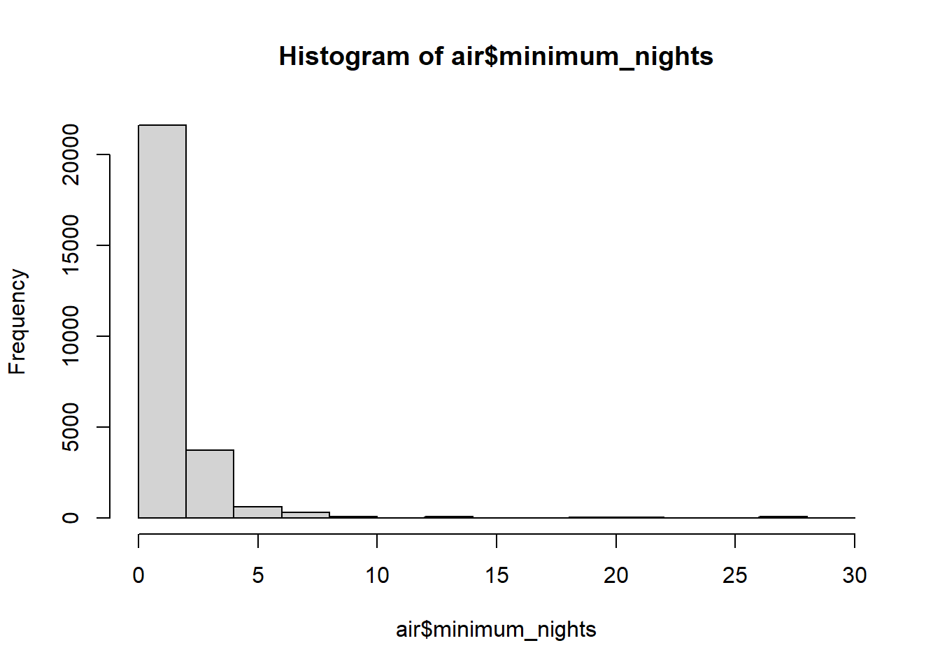
Your task: Can you go and fix the column maximum_nights I won’t tell you what value to choose is extreme and what to replace with, but it should be something that makes sense in the context of the data.
6.5.2 Replace missing value with assumed value
Our columns cleaning_fee and security_deposit both have a bunch of NA values. I’m going to assume the reason why they’re missing is because the agent doesn’t have a cleaning fee or security deposit, and thus the value should be 0 but they didn’t fill it in when listing.
We could use an ifelse to replace our NA values, but the perk to NA values is that R can rapidly find them and do things with them - in this case replace them!
Here’s a base R way to use the function is.na(). So we can use the same syntax that we used to filter rows in our R Refresher lesson. But, instead where we were filtering by asking something like air$security_deposit >= 10, which would return T or F if the condition is met, we are going to use is.na() to ask T or F if the value in that row is NA. One little thing - we’re assigning zero to the every value where that condition is TRUE, so the slicing actually falls right of the arrow here.
Here’s a quick example of is.na() in action
xyz <- c(1,2,3, NA, 4, 5, NA)
is.na(xyz)
## [1] FALSE FALSE FALSE TRUE FALSE FALSE TRUENow to replace
air$security_deposit[is.na(air$security_deposit)] <- 0
# "in air$security_deposit, if there is an NA in security_deposit, replace with 0"
summary(air$security_deposit) # looks good!
## Min. 1st Qu. Median Mean 3rd Qu. Max.
## 0.0 0.0 0.0 142.4 250.0 999.0Your task Go and fix the cleaning_fee column. Let’s assuming that NA values should be 0.
6.5.3 Imputing missing values
Imputing is a process where you make some statistical estimate about the nature of the missing value. We’ll do the simplest form of imputation here by just replacing NA values with the mean/median of that column.
Let’s look at a summary of bedrooms.
##    Min. 1st Qu.  Median    Mean 3rd Qu.    Max.    NA's
##   0.000   1.000   1.000   1.473   2.000  24.000       7
We see that there are only 6 NA values and the median is 1 and the mean is just a bit above. Let’s replace our NA values with the median. In this case the condition we’re checking in our ifelse is if the value in air$bedrooms is NA using is.na()
A quick note - when asking for the median() or mean() of a column you need to tell R what you want to do with the NA values. If there are NA values in there R will return NA back as you can’t calculate with them. If you specify na.rm=TRUE, R knows to ignore them in the calculate (na.rm just mean ‘remove na?’). Let’s see an example
xyz <- c(1,2,3, NA, 4, 5, NA)
mean(xyz)
## [1] NAmean(xyz, na.rm = TRUE)## [1] 3OK, do it with bedrooms now.
air$bedrooms <- ifelse(is.na(air$bedrooms), median(air$bedrooms, na.rm=TRUE), air$bedrooms)
summary(air$bedrooms) # check - looks good!
## Min. 1st Qu. Median Mean 3rd Qu. Max.
## 0.000 1.000 1.000 1.473 2.000 24.000Again, this is the simplest version of imputing. There are more complex methods where it evaluates the data using a linear regression model and imputes the predicted value for the missing one. Say for example if you knew someone’s height but their weight was NA in a dataframe. You could use the weight ~ height regression model from the previous lesson to provide a smarter estimate!
Your task: Go and fix the bathrooms column. What should you replace the NA values with?
6.5.4 Dropping columns
There’s no firm rule on when to just drop a whole column. Still, in this case we can can see that 97.0113% of our square_feet column are NA values.
##    Min. 1st Qu.  Median    Mean 3rd Qu.    Max.    NA's
##     0.0   550.0   600.0   777.1  1000.0  5500.0   25838
## [1] 97.01134Let’s just drop it as imputing would be pointless as we don’t have nearly enough data to make an informative estimate with.
air <- air %>%
  select(-square_feet)
6.6 Rescaling and changing distribution
Sometimes in preprocessing you need to change the scaling or alter the distribution of your features. This is because some model types that we’ll be working with are very sensitive to differences in feature scale. For example, a feature that ranges from 0-70,000 will take priority over one that ranges from 0-70 even if the variance is the same and they’re equally important.
Other times the distribution of the feature is just off and using it as continuous doesn’t make sense.
6.6.1 Converting to binary
Let’s take a look at a histogram of host_response_rate
hist(air$host_response_rate)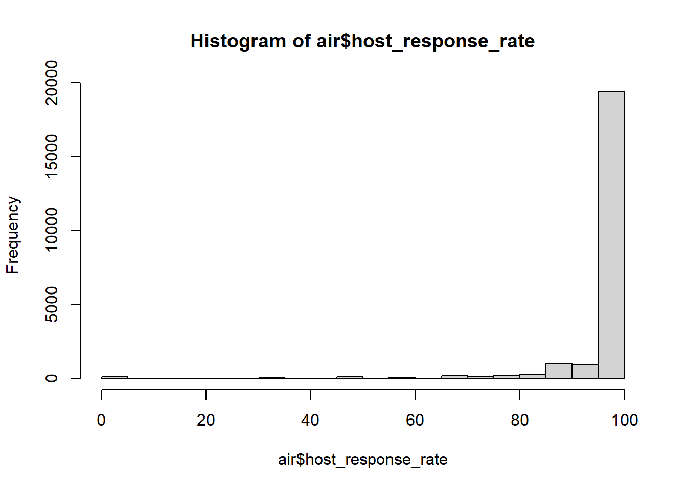 These data are clearly not normally distributed, and it might not make sense to really use them as a continuous feature. Instead, it might be worth just making the data binary and considering them as ‘good responders’ and ‘bad responders’. We could define a good responder as someone who responds say 90% of the time, and everything else as a bad responder.
We can create a whole new column and use an ifelse to define the new values
# Create a new column host_responder
# When host_response rate is greater than 90 then fill with 'good_responder'
# Otherwise they're a 'bad_responder'
air$host_responder <- ifelse(air$host_response_rate >= 90, 'good_responder', 'bad_responder')
glimpse(air)# check
## Rows: 26,634
## Columns: 20
## $ price <dbl> 50, 117, 80, 150, 35, 215, 99, 99, 145, 99, ...
## $ cleaning_fee <dbl> 15, 35, 0, 95, 50, 100, 75, 80, 55, 150, 100...
## $ security_deposit <dbl> 0, 0, 0, 0, 200, 0, 0, 200, 0, 300, 300, 0, ...
## $ cancellation_policy <chr> "strict_14_with_grace_period", "moderate", "...
## $ minimum_nights <dbl> 2, 2, 2, 4, 2, 4, 1, 1, 1, 1, 2, 3, 3, 1, 1,...
## $ maximum_nights <dbl> 89, 60, 60, 60, 365, 120, 365, 365, 365, 300...
## $ bedrooms <dbl> 1, 3, 1, 1, 1, 2, 2, 0, 2, 2, 3, 1, 1, 2, 1,...
## $ bathrooms <dbl> 1.0, 1.0, 1.0, 1.0, 1.0, 1.0, 2.0, 1.0, 1.0,...
## $ accommodates <dbl> 1, 7, 2, 4, 2, 4, 4, 3, 7, 6, 6, 2, 2, 6, 4,...
## $ bed_type <chr> "real_bed", "real_bed", "futon", "real_bed",...
## $ room_type <chr> "private_room", "entire_home_apt", "entire_h...
## $ property_type <chr> "Condominium", "Apartment", "Apartment", "Ap...
## $ city <chr> "Chicago", "Chicago", "Chicago", "Chicago", ...
## $ host_identity_verified <lgl> TRUE, TRUE, FALSE, TRUE, TRUE, TRUE, TRUE, T...
## $ host_is_superhost <lgl> TRUE, TRUE, FALSE, FALSE, FALSE, FALSE, FALS...
## $ host_response_time <chr> "within an hour", "within an hour", "within ...
## $ host_response_rate <dbl> 100, 100, 100, 89, 93, 89, 100, 100, 100, 10...
## $ review_scores_rating <dbl> 100, 96, 92, 92, 85, 89, 93, 85, 86, 86, 89,...
## $ number_of_reviews <dbl> 149, 368, 338, 35, 38, 9, 9, 37, 178, 44, 47...
## $ host_responder <chr> "good_responder", "good_responder", "good_re...6.6.2 Rescaling features
As mentioned above, you sometimes must rescale features so a model fits correctly. Scaling features also helps with interpreting your model output. One common way is to do this is to rescale all your features so they have a mean of 0 and a standard deviation of one using the following formula: \[ x_{scaled} = \frac{x - \overline{x}}{sd_{x}}\]
6.6.2.1 Demonstrating how to scale
Let’s do a quick example of how to scale. Let’s make a normal distribution of prices using the following code and then make a histogram. We can see that the mean falls around 100 as we specified, and that 95% of the data will fall within +/- 20 as we said the SD should be 20.
price <- rnorm(mean = 100, sd = 20, n = 100)
hist(price)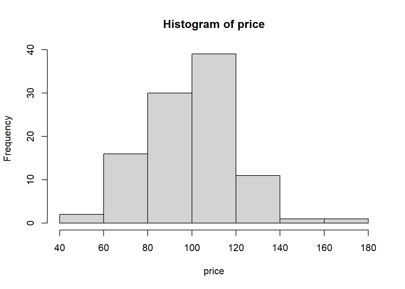
But we can scale it to have a mean of zero and standard deviation to be one using the above formula and a use of the sd() function. Note how our data are now centered around 0 and 95% of our data fall into +/- one unit.
price_scaled <- (price - mean(price))/sd(price)
hist(price_scaled)
We can also use a convient scale() function to do this for us.
price_scaled_2 <- scale(price)
hist(price_scaled_2)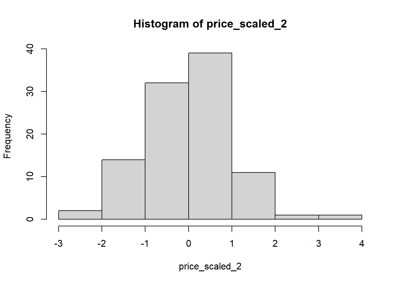
6.6.2.2 Why scale?
The perk to this scaling is it makes it so that your regression features all on the same scale, and thus your \(\beta\) coefficients tell you how much your target changes for one \(SD\) change in the feature. Let’s see an example.
First, let’s understand how cleaning_fee and accommodates influence price. You might think that those who have a high cleaning fee charge less (they’re padding their price with cleaning fees). Similarly, you’d assume that larger places can charge more.
Looking at our summary we see really different betas for our two features, but both are highly significant. Is one more important than the other? It’s sorta hard to say. They’re on different scales (cleaning_fee is related to dollars, where accommodates considers number of people that’ll fit).
summary(lm(price ~ cleaning_fee + accommodates, data = air))##
## Call:
## lm(formula = price ~ cleaning_fee + accommodates, data = air)
##
## Residuals:
## Min 1Q Median 3Q Max
## -475.12 -52.42 -20.34 21.81 888.75
##
## Coefficients:
## Estimate Std. Error t value Pr(>|t|)
## (Intercept) 32.68330 1.51005 21.64 <2e-16 ***
## cleaning_fee 0.74480 0.01303 57.17 <2e-16 ***
## accommodates 18.16350 0.35514 51.15 <2e-16 ***
## ---
## Signif. codes: 0 '***' 0.001 '**' 0.01 '*' 0.05 '.' 0.1 ' ' 1
##
## Residual standard error: 118.5 on 23569 degrees of freedom
## (3062 observations deleted due to missingness)
## Multiple R-squared: 0.304, Adjusted R-squared: 0.3039
## F-statistic: 5147 on 2 and 23569 DF, p-value: < 2.2e-16Let’s wrap the scale() function around each feature and look again.
summary(lm(price ~ scale(cleaning_fee) + scale(accommodates), data = air))##
## Call:
## lm(formula = price ~ scale(cleaning_fee) + scale(accommodates),
## data = air)
##
## Residuals:
## Min 1Q Median 3Q Max
## -475.12 -52.42 -20.34 21.81 888.75
##
## Coefficients:
## Estimate Std. Error t value Pr(>|t|)
## (Intercept) 159.1936 0.7728 205.99 <2e-16 ***
## scale(cleaning_fee) 49.9089 0.8730 57.17 <2e-16 ***
## scale(accommodates) 43.6741 0.8539 51.15 <2e-16 ***
## ---
## Signif. codes: 0 '***' 0.001 '**' 0.01 '*' 0.05 '.' 0.1 ' ' 1
##
## Residual standard error: 118.5 on 23569 degrees of freedom
## (3062 observations deleted due to missingness)
## Multiple R-squared: 0.304, Adjusted R-squared: 0.3039
## F-statistic: 5147 on 2 and 23569 DF, p-value: < 2.2e-16So this is in a lot of ways easier to understand as now one unit is one \(SD\). In other words, our beta coefficients say how much the target will change for one \(SD\) in each feature! So we see that each actually has a similar effect when you consider an equal change (1 \(SD\)) in the feature!
It’s worth noting that our \(RSE\), \(R^2\), and \(p\)-value didn’t change… in regression models scaling doesn’t influence the model fit itself, just how you interpret coefficients!
6.7 One hot encoding
What the heck is one hot encoding? Well, it sounds complicated but it’s really just a way to represent categorical data using a series of binary features. We’ve already fit binary features in regression models (did it rain - yes or no; is the person a smoker or not). Those just have two levels, and thus can be represented with a simple 0 and 1.
What happens if we have more than two levels and each level is it’s on category? We have a bunch of features like that here in our AirBnB data. For example city has four clear categories:
## [1] "Chicago" "Portland" "Seattle" "San_Francisco"But models can’t directly fit features with multiple categories like this. Instead you need to convert it to a series of binary variables (also known as dummy variables) where each one ‘asks’ if the observation is part of that category. For example, city can be represented as four features in your data frame:
- city_is_chicago: yes or no
- city_is_Seattle: yes or no
- city_is_San_Francisco: yes or no
- city_is_Portland: yes or no
You could write code to do this, but of course someone has already made a handy function for us! Go install the package caret and then load it.
## Loading required package: lattice##
## Attaching package: 'caret'## The following object is masked from 'package:purrr':
##
## liftWe can use the wonderful dummyVars() function to take a single feature with multiple categorical levels and expand it into several dummy features. There are a couple steps to this.
Let’s make dummies for city. First, you make a dummies object using the dummyVars() feature. You need to specify the feature you want to convert using the syntax ~ feature_to_convert. You can use a + if you want to convert multiple at once. You also need to tell it your data using data = and then specify fullRank = TRUE
my_dummies <- dummyVars( ~ city, data = air, fullRank = TRUE)Next you need to use this object to predict the values of the newly created columns. You can use the predict() function. Inside you specify what object you’re using to predict (in this case my_dummies) and then the data you want to predict from (newdata = air).
my_dummies_pred <- predict(my_dummies, newdata = air)my_dummies_pred is a data frame if dummy variables…
##   cityPortland citySan_Francisco citySeattle
## 1            0                 0           0
## 2            0                 0           0
## 3            0                 0           0
## 4            0                 0           0
## 5            0                 0           0
## 6            0                 0           0
This isn’t much use as our target is in our original air data frame. Luckily we can just join these new dummy variables onto air using the function cbind(). All cbind means is ‘column bind’ or ‘bind these columns together’.
air <- cbind(air, my_dummies_pred) # bind our two data frames
glimpse(air) # check
## Rows: 26,634
## Columns: 23
## $ price <dbl> 50, 117, 80, 150, 35, 215, 99, 99, 145, 99, ...
## $ cleaning_fee <dbl> 15, 35, 0, 95, 50, 100, 75, 80, 55, 150, 100...
## $ security_deposit <dbl> 0, 0, 0, 0, 200, 0, 0, 200, 0, 300, 300, 0, ...
## $ cancellation_policy <chr> "strict_14_with_grace_period", "moderate", "...
## $ minimum_nights <dbl> 2, 2, 2, 4, 2, 4, 1, 1, 1, 1, 2, 3, 3, 1, 1,...
## $ maximum_nights <dbl> 89, 60, 60, 60, 365, 120, 365, 365, 365, 300...
## $ bedrooms <dbl> 1, 3, 1, 1, 1, 2, 2, 0, 2, 2, 3, 1, 1, 2, 1,...
## $ bathrooms <dbl> 1.0, 1.0, 1.0, 1.0, 1.0, 1.0, 2.0, 1.0, 1.0,...
## $ accommodates <dbl> 1, 7, 2, 4, 2, 4, 4, 3, 7, 6, 6, 2, 2, 6, 4,...
## $ bed_type <chr> "real_bed", "real_bed", "futon", "real_bed",...
## $ room_type <chr> "private_room", "entire_home_apt", "entire_h...
## $ property_type <chr> "Condominium", "Apartment", "Apartment", "Ap...
## $ city <chr> "Chicago", "Chicago", "Chicago", "Chicago", ...
## $ host_identity_verified <lgl> TRUE, TRUE, FALSE, TRUE, TRUE, TRUE, TRUE, T...
## $ host_is_superhost <lgl> TRUE, TRUE, FALSE, FALSE, FALSE, FALSE, FALS...
## $ host_response_time <chr> "within an hour", "within an hour", "within ...
## $ host_response_rate <dbl> 100, 100, 100, 89, 93, 89, 100, 100, 100, 10...
## $ review_scores_rating <dbl> 100, 96, 92, 92, 85, 89, 93, 85, 86, 86, 89,...
## $ number_of_reviews <dbl> 149, 368, 338, 35, 38, 9, 9, 37, 178, 44, 47...
## $ host_responder <chr> "good_responder", "good_responder", "good_re...
## $ cityPortland <dbl> 0, 0, 0, 0, 0, 0, 0, 0, 0, 0, 0, 0, 0, 0, 0,...
## $ citySan_Francisco <dbl> 0, 0, 0, 0, 0, 0, 0, 0, 0, 0, 0, 0, 0, 0, 0,...
## $ citySeattle <dbl> 0, 0, 0, 0, 0, 0, 0, 0, 0, 0, 0, 0, 0, 0, 0,...But wait, how come we only have three dummy variables when there were four unique levels to city? Well, the same reason a simple binary (i.e. smoker vs. not) doesn’t have two columns (i.e. yes_smoker & no_smoker). If you include a column for every level and fit all those features you have no reference to compare against. Thus you drop one and that is your baseline. In the case of us encoding city we can see that Chicago was dropped, and thus it is our reference to compare the other features against. Let’s fit a model to make this more clear.
city_mod <- lm(price ~ cityPortland + citySan_Francisco + citySeattle, data = air)
summary(city_mod)
##
## Call:
## lm(formula = price ~ cityPortland + citySan_Francisco + citySeattle,
## data = air)
##
## Residuals:
## Min 1Q Median 3Q Max
## -195.30 -77.48 -38.30 29.38 878.38
##
## Coefficients:
## Estimate Std. Error t value Pr(>|t|)
## (Intercept) 137.484 1.630 84.350 < 2e-16 ***
## cityPortland -16.865 2.628 -6.418 1.4e-10 ***
## citySan_Francisco 57.820 2.375 24.341 < 2e-16 ***
## citySeattle 25.347 2.261 11.211 < 2e-16 ***
## ---
## Signif. codes: 0 '***' 0.001 '**' 0.01 '*' 0.05 '.' 0.1 ' ' 1
##
## Residual standard error: 139.6 on 26379 degrees of freedom
## (251 observations deleted due to missingness)
## Multiple R-squared: 0.03511, Adjusted R-squared: 0.035
## F-statistic: 319.9 on 3 and 26379 DF, p-value: < 2.2e-16So, all of our \(\beta\) estimates are relative to Chicago. Portland is cheaper, while San Francisco and Seattle are higher. Clearly based on the \(R^2\) there is still a lot of price variation to explain, but city does matter!
A quick note - you’ll see that if you just fit a simpler not encode model of lm(price ~ city, data = air) that you get the same output. Why is this? Well, R is doing the one hot encoding for you behind the scenes! That’s great and all, but many models won’t do it for you, so it’s good to incorporate this into your workflow.
Your task: Go and one hot encode bed_type, run a model with the bed types, and then make some inference on how the type of bed in the listing influences price.