9.3 CIs and tests for mean differences (paired data)

Guirao et al. (2017) examined the difference between 2-minute walk test score (2MWT) for \(10\) patients before and after receiving a prosthetic implant. (The 2MWT measures how far participants can walk in two minutes, in metres.)
The 2MWT for ten amputees with and without an implant are shown in Fig. 9.1. The researchers asked:
For this type of amputee, is the mean 2MWT improved (i.e., longer distances walked) after using the implant?
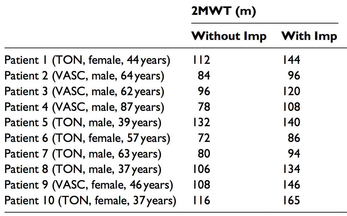
FIGURE 9.1: Two-minute Walk Times (2MWT) for \(10\) patients with implants (With Imp) and without implants (Without Imp), in metres
- What type of RQ is implied: descriptive, relational, repeated-measures or correlational?
- What do \(\mu_d\) and \(\bar{d}\) represent in this context?
- Explain why these data should be analysed as paired data.
- Compute the changes in 2MWT for each patient.
- Although it doesn't really matter, why does it probably makes more sense to compute the With Imp values minus the Without Imp values?
- Using the statistics mode on your calculator, compute the sample mean difference \(\bar{d}\) and the sample standard deviation of the differences \(s_d\).
- Compute the standard error of the mean difference \(\text{s.e.}(\bar{d})\).
- Explain the meaning of the standard error of the mean difference in this context.
- If another sample of ten subjects were studied, would the same sample mean difference \(\bar{d}\) be computed? How much variation would be expected in the sample mean differences found from different samples?
- Draw the approximate sampling distribution of \(\bar{d}\) that shows how the value of \(\bar{d}\) varies.
- Compute an approximate \(95\)% confidence interval for the population mean difference in 2MWT.
Which of the following is the correct null hypothesis for this RQ? Why are the others incorrect? Is the test one- or two-tailed? What is the alternative hypothesis?
- \(\mu_{\text{Without Implant}} = \mu_{\text{With implant}}\)
- \(\mu_{\text{Difference}} = 0\)
- \(\mu_{\text{Difference}} > 0\)
- \(\mu_{\text{Without Implant}} = 0\)
- \(\mu_{\text{With implant}} = 0\)
- \(\mu_{\text{Without Implant}} < \mu_{\text{With implant}}\)
- \(\mu_{\text{Difference}} < 0\)
- \(\mu_{\text{Without Implant}} < 0\)
- \(\mu_{\text{With implant}} > 0\)
Write down the value of the \(t\)-statistic, then estimate the \(P\)-value for testing the hypotheses (using Fig. 9.2).
Explain why the \(t\)-score from jamovi is a negative value, but the \(t\)-score from SPSS (Fig. 9.4) is a positive value.
Write a statement that communicates the result of the test.
What conditions must be met for this test to be valid?
Is it reasonable to assume the assumptions are satisfied? How does Fig. 9.3 help, if at all?
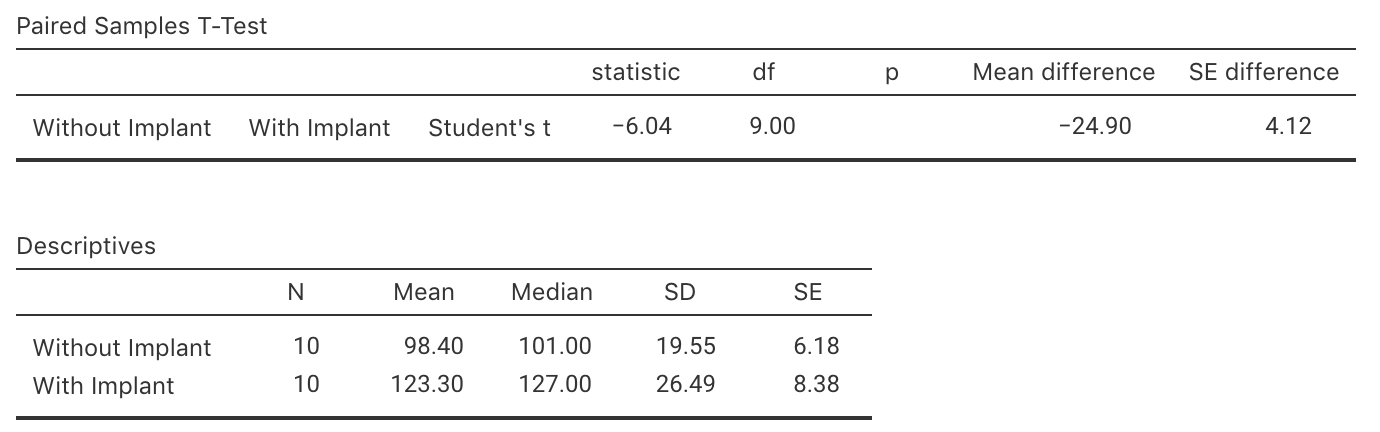
FIGURE 9.2: Output from jamovi for the 2MWT example, partially edited
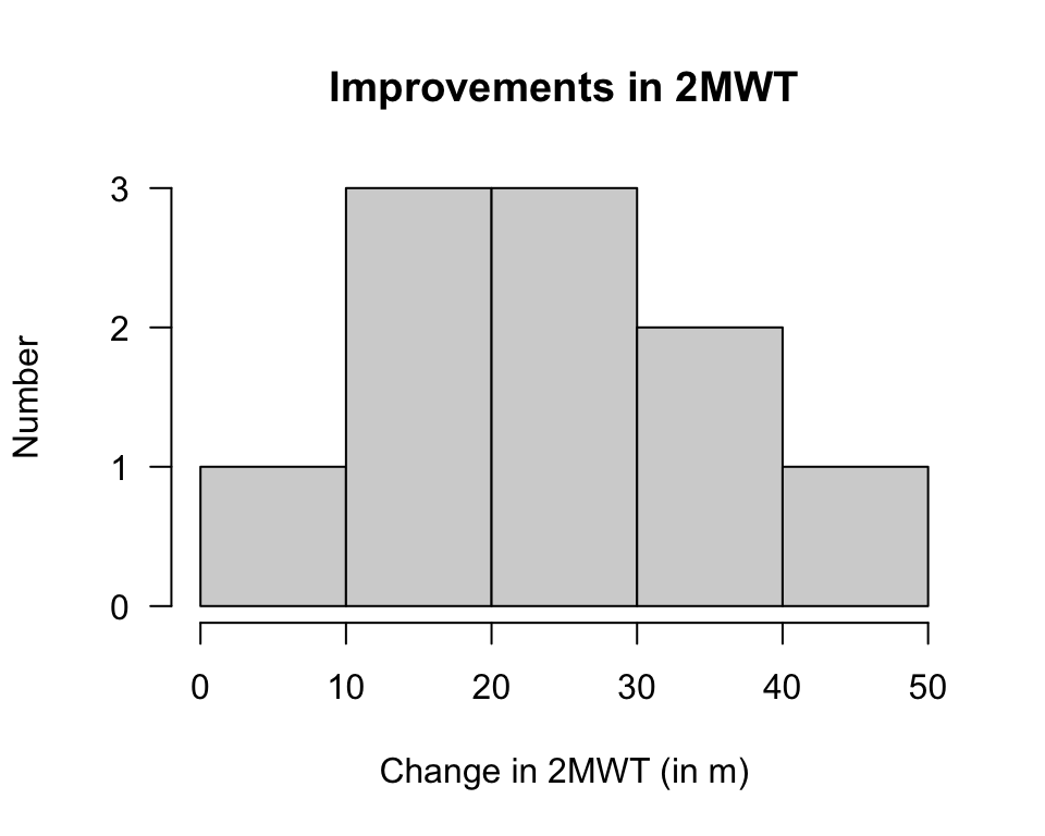
FIGURE 9.3: Histogram of differences for the increases in 2MWT with implant
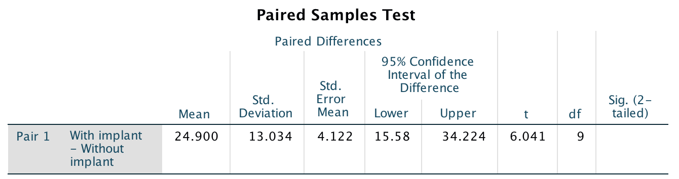
FIGURE 9.4: Output from SPSS for the 2MWT example, partially edited