9.6 Optional questions
These questions are optional; e.g., if you need more practice, or you are studying for the exam. (Answers appear in Sect. A.9.)
9.6.1 (Optional) CIs and tests for paired samples
This question has a video solution in the online book, so you can hear and see the solution.
After a number of runners collapsed near the finish of the Tyneside annual Great North Run, researchers decided to study the role of \(\beta\) endorphins as a factor in the collapses. (\(\beta\) endorphins are a peptide which suppress pain.)
A study (Dale et al. 1987) examined what happened with plasma \(\beta\) endorphins during fun runs: how much do the concentrations change, on average? The researchers recorded the plasma \(\beta\) concentrations in fun runners (participating in the Tyneside Great North Run). Eleven runners (who did not collapse) had their plasma \(\beta\) concentrations measured (in pmol/litre) before and after the race (Table 9.1.)
| Before race | After race | Increase |
|---|---|---|
| \(\phantom{0}4.3\) | \(29.6\) | \(25.3\) |
| \(\phantom{0}4.6\) | \(25.1\) | \(20.5\) |
| \(\phantom{0}5.2\) | \(15.5\) | \(10.3\) |
| \(\phantom{0}5.2\) | \(29.6\) | \(24.4\) |
| \(\phantom{0}6.6\) | \(24.1\) | \(17.5\) |
| \(\phantom{0}7.2\) | \(37.8\) | \(30.6\) |
| \(\phantom{0}8.4\) | \(20.1\) | \(11.7\) |
| \(\phantom{0}9.0\) | \(21.9\) | \(12.9\) |
| \(10.4\) | \(14.2\) | \(\phantom{0}3.8\) |
| \(14.0\) | \(34.6\) | \(20.6\) |
| \(17.8\) | \(46.2\) | \(28.4\) |
The 'usual' value for \(\beta\) endorphines is usually less than about \(11\) pmol/litre.
What do \(\mu_d\) and \(\bar{d}\) represent in this context?
Explain why these data should be analysed as mean differences.
Compute the changes in plasma \(\beta\) endorphin concentration during the run (i.e. the 'differences'). (Although it doesn't really matter, why does it probably makes more sense to compute the after values minus the before values?)
Using the statistics mode on your calculator, compute the sample mean difference \(\bar{d}\) and the sample standard deviation of the differences.
Compute the standard error of the mean difference. Explain what this means in this context.
If another sample of eleven runners were studied, would the same sample mean difference be computed? How much variation would be expected in the sample means found from different samples?
Compute an approximate \(95\)% CI for the population mean difference in plasma \(\beta\) concentrations.
Which of the following is the correct null hypothesis for this question? Why are the others incorrect? Is the test one- or two-tailed?
- \(\mu_{\text{Before}} = \mu_{\text{After}}\)
- \(\mu_{\text{Difference}} = 0\)
- \(\mu_{\text{Before}} = 0\)
- \(\mu_{\text{After}} = 0\)
- \(\mu_{\text{Before}} < \mu_{\text{After}}\)
- \(\mu_{\text{Difference}} > 0\)
- \(\mu_{\text{Before}} < 0\)
- \(\mu_{\text{After}} > 0\)
Write down the value of the \(t\)-statistic, then estimate the \(P\)-value (using the \(68\)--\(95\)--\(99.7\) rule).
Write a statement that communicates the result of the test.
What conditions must be met for this test to be valid?
Is it reasonable to assume the assumptions are satisfied? How does the histogram in Fig. 9.9 help, if at all?
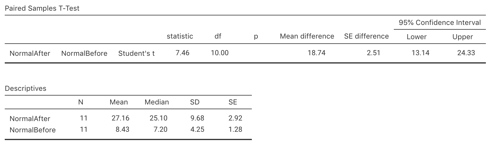
FIGURE 9.8: Output from jamovi for the fun run example, partially edited
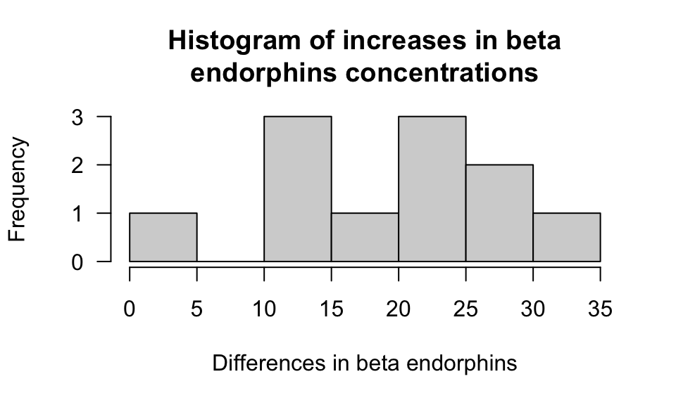
FIGURE 9.9: Histogram of differences for the fun run example
9.6.2 (Optional) CI and test for mean differences (paired data)
Wave power has been considered as a source of energy since 1890, but the engineering necessary to successfully and practically harness this energy is complex.
To understand one method of harnessing this energy, one study (Hand et al. 1996) examined the bending stress (in Newton--metres) in part of a device used to generate electricity from wave power. Two different mooring types were compared (Table 9.2) in \(n = 18\) different sea states.
| Method 1 | Method 2 | Differences |
|---|---|---|
| 2.23 | 1.82 | 0.41 |
| 2.55 | 2.42 | 0.13 |
| 7.99 | 8.26 | -0.27 |
| 4.09 | 3.46 | 0.63 |
| 9.62 | 9.77 | -0.15 |
| 1.59 | 1.4 | 0.19 |
| 8.98 | 8.88 | 0.1 |
| 0.82 | 0.87 | -0.05 |
| 10.83 | 11.2 | -0.37 |
| 1.54 | 1.33 | 0.21 |
| 10.75 | 10.32 | 0.43 |
| 5.79 | 5.87 | -0.08 |
| 5.91 | 6.44 | -0.53 |
| 5.79 | 5.87 | -0.08 |
| 5.5 | 5.3 | |
| 9.96 | 9.82 | |
| 1.92 | 1.69 | |
| 7.38 | 7.41 |
- Explain why these data should be analysed as mean differences.
- Compute the sample differences (most have been done for you).
- Using the statistics mode on your calculator, compute the sample mean and the sample standard deviation of these differences.
- Compute the standard error of the mean difference. What does this value mean?
- Compute an approximate \(95\)% CI for the population mean difference in two methods.
- Conduct a hypothesis test to determine if the mean bending stress is different between the two methods.
- What conditions must be met for this CI and test to be statistically valid?
- Is it reasonable to assume the CI and test are statistically valid?
Draw a stem-and-leaf plot to check.
9.6.3 (Optional) CI for differences between two means
This question has a video solution in the online book, so you can hear and see the solution.
In 2011, Eagle Boy's Pizza ran a campaign (Dunn 2012) that claimed that Eagle Boy's pizzas were larger than Domino's large pizzas. Eagle Boy's made the data behind the campaign publicly available.
Each sample contained similar pizzas types (the three toppings were: supreme, Hawaiian, meat-lovers; the three base types were deep, thin, mid).
Some output from a sample of \(125\) of Eagle Boys' and Domino's large pizzas is shown in Fig.
9.10 (jamovi).
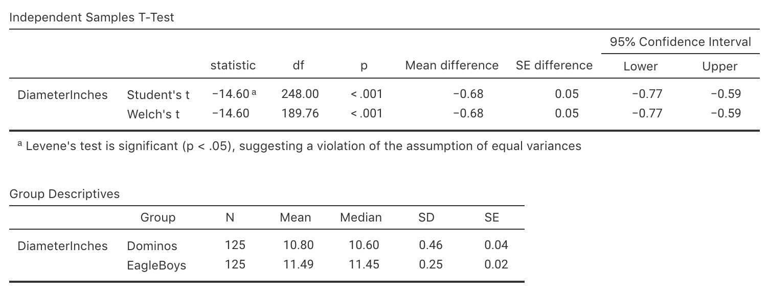
FIGURE 9.10: Summary statistics for the diameter of Eagle Boy's and Domino's large pizzas, from jamovi
Explain whether the study is observational or experimental (true or quasi).
Identify the type of research question is being answered: descriptive, relational, repeated-measures or correlational? Explain.
Two students are arguing about this study. One claims that the study compares two independent samples, because the pizzas have come from two different companies completely. The other student argues that the study has paired samples, because each store has the same types of pizzas in the sample (e.g. both have supreme, Hawaiian and meat-lovers pizzas).
With whom do you agree? Why?
Write down the CI to estimate the difference in population means.
What does the right panel of Fig. 9.11 communicate?
Conduct a hypothesis tests to compare the two brands.
What condition must hold for the CI to be statistically valid?
Is it reasonable to assume these conditions are satisfied? (You may need to refer Fig. 9.11.)
Eagle Boy's claimed that their pizzas are 'larger' than Domino's pizzas. Do you agree or disagree?
Why? What other information would be helpful for answering this question?
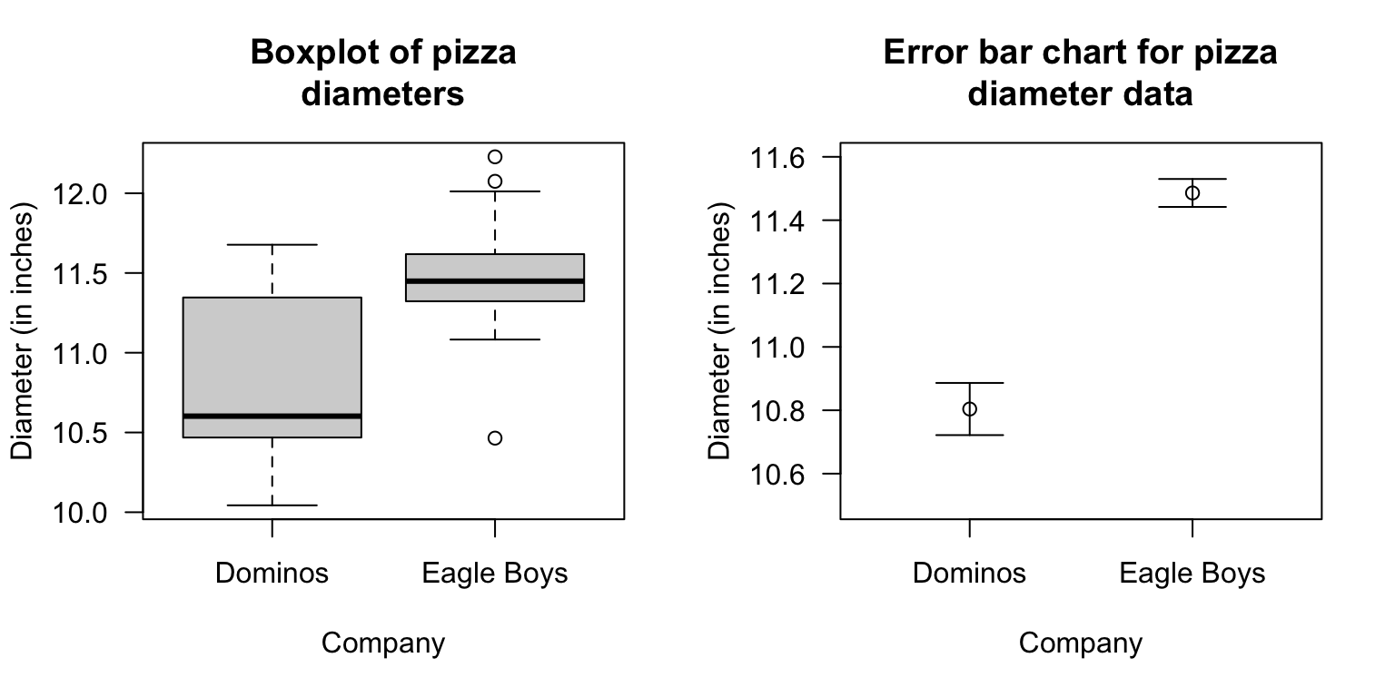
FIGURE 9.11: Boxplot (left panel) and error-bar chart (right panel) for the pizza size data
9.6.4 (Optional) Tests for comparing the mean from two independent samples
(Answers available in Sect. A.10)
This question has a video solution in the online book, so you can hear and see the solution.
Batteries are expensive, so comparing the performance of expensive and cheap batteries is helpful.
A test on the lifetime of batteries (Lindström 2011) compared the time for two brands of \(1.5\) volt batteries to reduce their voltage to \(1.0\) volts under standard testing conditions.
The times (in hours) for nine Energizer Max batteries and nine ALDI brand batteries (Ultracell) are shown in Table 9.3.
| Energizer | 7.58 | 7.46 | 7.46 | 7.59 | 7.46 | 7.52 | 6.83 | 6.89 | 7.45 |
| Ultracell | 7.5 | 7.48 | 7.47 | 7.48 | 7.48 | 7.41 | 7.47 | 6.96 | 7.48 |
Write the hypotheses for testing the research question of interest. Is the test one- or two-tailed?
Explain the meaning of the standard error of the mean in this context.
The software output for the analysis is shown in Fig. 9.12. Determine the value of the \(t\)-statistic and the \(P\)-value for testing the hypotheses.
Write a statement that communicates the result of the test.
What conditions must be met for this test to be valid?
Is it reasonable to assume the assumptions are satisfied?
What did you learn from this study?
At the time of this analysis, a four-pack of the Ultracell Max batteries cost $2.49 from ALDI online, while a four pack of Energizer Max from Woolworths online cost $5.97 on special (usually $8.01)3.
On the basis of this information, would you be prepared to try the Ultracell batteries? Explain your reasoning.
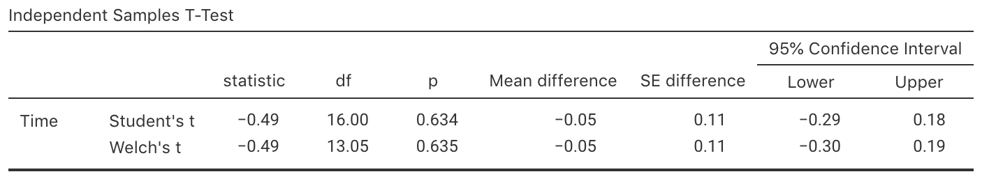
FIGURE 9.12: Output from jamovi for the battery data
References
Data from 05 September 2012.↩︎