4 Assumptions and confidence in estimated coefficients
Abstract
This chapter discusses assumptions needed for OLS estimates to be valid for making inferences about the population relationship. The chapter discusses how to conduct hypothesis tests and calculate confidence intervals for the estimated coefficients. Keywords: Hypothesis test, confidence interval, bias, least-squares
4.1 Inference in regression analysis
We continue with the example, introduced in the previous chapter, of estimating the effects of education attainment on earnings, at the individual level. The previous chapter introduced the idea of a single variable regression analysis. We introduced the ordinary least squares method, and we estimated parameters for a best fit line by calculating the values that minimized the sum of squared deviations. In doing so, we mentioned several assumptions. In this chapter we elaborate on those assumptions and introduce others that are important for the analysis. The idea is that a researcher would determine or assess whether the line estimated, using the method of OLS, for a sample of data that has been randomly selected from the population of interest, is a reasonable estimate for the population relationship, by examining the validity or credibility of the various assumptions. If the assumptions are unlikely to be valid, there is no reason to think the OLS estimated coefficients are especially valid. More complex estimation methods, and other assumptions, may be needed for valid estimation.
Using the language from Chapter 2, we would like to make a valid inference about the population relationship, from the analysis of the sample relationship. This chapter addresses the question of how much confidence to have in the estimates from OLS, given that we estimate them from a sample of data from the population. Another sample would generate different estimates. If the sample size were small, then two samples might generate very different estimates of the regression coefficients. It should be obvious that we would have little confidence in a regression line estimated from a sample of six observations. We should, though, make precise what we might mean when we talk about confidence in the estimated coefficients. The methods introduced here form the basis for addressing similar questions in more complex regression analysis.
4.2 Assumptions typically made when doing regression analysis
A well-known joke in academia is the following. A physicist, an engineer and an economist are stranded of a desert island. They find a can of corn. They want to open it, but how? The physicist says: “Let’s start a fire and place the can inside the flames. It will explode and then we will all be able to eat.” “Are you crazy?” says the engineer. “All the corn will burn and scatter, and we’ll have nothing. And we don’t have a fire. We’ll build a three-rock vise underneath the coconut tree to hold the can, and some of the falling coconuts will hit the can, and the metal will weaken, and we’ll be able to crack the can open.” “I have a better idea,” states the economist. “Let’s just assume we have a can opener.” The joke is a dig at economists who often try to understand complex questions by pretending, or assuming, that the questions are simple rather than complex.
The problem in introductory econometrics is to estimate a valid and credible relationship between an explanatory variable and an outcome variable. The word “valid” is usually associated with the considerations of statistical analysis (is the analyst following proper statistical procedures for inference) while the word “credible” is usually associated with whether the estimated relationship is likely to be causal, or merely correlational.
Here are five key assumptions that make the method of OLS more likely to be valid and credible. There are other assumptions lurking in the background of our analysis that we shall mention in subsequent chapters, so this list of five is not exhaustive. • The direction of causality is from \(X\) to \(Y\) • The true relationship, or population relationship, is linear • The probability of selecting a sample with extreme outliers of either \(X\) or \(Y\) (or both) is low • Other factors affecting the outcome are uncorrelated with the explanatory variable • The data is a random sample of observations from the population of interest, and observations are independent and identically distributed (i.i.d.) We recognize that validity or credibility is always a judgment call: there are no absolute criteria of what is valid; the community of researchers generates an evolving consensus standard that is occasionally disputed.
If the five assumptions above hold, OLS is a very good representation of the causal relationship in the population: it generates an unbiased (“on target”) estimate of the parameter of interest and the estimate is likely to be precise (in a sense to be explained below). See Box 1 for an algebraic proof that makes clear what exactly is meant by “unbiased.”
By minimizing the vertical “mistakes,” OLS captures the idea of the predicted or expected \(Y\) conditional on the value of \(X\). There are alternative ways to find the “best-fitting” line, though. One method, for example, minimizes the sum of the absolute value of deviations. Another might apply OLS but with a sample that drops outliers. These alternative methods are explored in more advanced econometrics textbooks. The convention in the social sciences is to use OLS if only as an important benchmark estimation method that virtually every social scientist understands, and so it acts as a common starting point for analysis.
4.2.1 Causality goes from X to Y
The mantra that “correlation does not imply causation” cannot be repeated often enough! OLS estimation on its own tells us nothing about causality. If we reverse the two variables in the regression equation, and have \(X\) be the outcome variable instead of the explanatory variable, we can still calculate a regression coefficient. How do we know whether \(X\) should be the explanatory variable or the outcome variable? We should properly be worried about our empirical example: perhaps individuals who anticipate high earnings later in life (because their parents are wealthy and will help them get good jobs) remain in school longer since they are less worried about the opportunity cost of education. The causality is reversed!
There will be more discussion later in the book about how to think about causality in the regression context. For now, we shall assume that the direction of causality is clear, and goes from \(X\) to \(Y\).
4.2.2 True relationship is linear and there should be a low probability of large outliers
As noted in the previous chapter, the goodness of fit measure \(R^2\) is one number to examine when evaluating a regression model. We might think that if the value of \(R^2\) were high (for example, above .80) then the model has done an excellent job. Consider, however, the data constructed by Anscombe (1973). Four small datasets, each with 11 observations of two variables \(X\) and \(Y\) . Anscombe constructed the data to generate roughly the same descriptive statistics (mean, standard deviation, median of \(X\) and \(Y\) are roughly the same in each of the four datasets, the same estimated regression coefficients, and roughly the same \(R^2\).
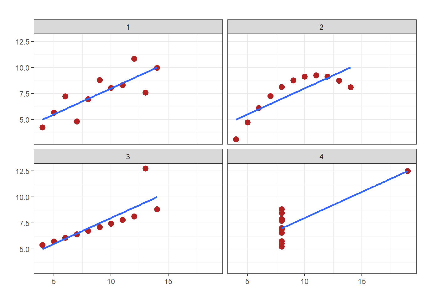
Figure 4.1: Four regression lines with same slope and \(R^2\) but very different patterns of data
As Figure 4.1 shows, the first scatter plot (top left) seems to have a well-fitted regression line and the deviations from the line appear to be random. The second scatter plot (top right) has a pattern of observations indicating a clear non-linear relationship between \(X\) and \(Y\) . The straight line fits very poorly, and yet has the same \(R^2\) as the first scatter plot. The third graph (bottom left) has all of the points on a straight line, but one outlier “pulls” the regression line away from the obvious fit. The plot illustrates the well-known problem that because OLS minimizes the square of the residuals, outliers have perhaps undue influence in determining the estimated coefficients. The fourth scatter plot (bottom right) suggests there is no relationship between \(X\) and \(Y\), but one single observation (again, an outlier) is enough to generate a regression line that looks just like the others and has a similar \(R^2\).
Anscombe’s intent in developing the dataset was to illustrate to data analysts the importance of graphing data and not just relying on estimated coefficients or other statistics. Graphing the data helps a researcher see whether some of the crucial assumptions of OLS are likely to be valid. In the case of the four plots, we might argue that in three of them (the non-linear patterned one and the two with outliers) the assumptions that make OLS a credible estimation strategy do not hold. We should use other estimation strategies in cases like these, where the relationship is likely non-linear, or where the probability of large outliers is likely.
In more advanced, mathematical treatments of econometrics, the assumption of low probability of very large outliers is made precise. The assumption is that the kurtosis of the distribution of each of the variables \(X\) and \(Y\) is finite (and not infinite). Kurtosis is a measure of the expected value of observations falling in the “tails” (the ends) of the distribution, and can be calculated, for the theoretical population distribution, as, \[kurtosis = \frac{E(Y - \mu_Y)^4}{\sigma_Y^4}\] or, for a sample, as, \[kurtosis = \frac{\sum\nolimits_{i=1}^N(Y_i - \overline{Y})^4/N}{s^4_Y}\] where \(\mu_Y\) is the population mean of the variable, \(\overline{Y}\) is the mean of the variable in the sample, \(s\) is the standard deviation (and \(\mu\) the standard deviation of the population distribution, and \(N\) is the number of data points. Kurtosis is a dimensionless number, and is non-negative. Note that the formula for a sample can be interpreted as follows: the numerator adds up deviations that are raised to the fourth power and divides by the sample size. The denominator takes the square root of the variance (deviations raised to the second power) and raises that to the fourth power. If the actual sum of deviations raised to the fourth power divided by \(N\) is quite a bit larger than the average deviation raised to the fourth power, the distribution is said to have high kurtosis. The standard normal distribution has kurtosis of 3, so in practice that is a value of reference. Some formula for kurtosis will automatically subtract 3 from the formula above.
In the previous chapter, we implicitly assumed that the relationship between education and earnings is a linear relationship. Later, we will relax this assumption, and see how we might estimate a non-linear relationship (e.g., a quadratic relationship, or an exponential relationship). We also assumed that the education variable had finite fourth moment (the deviations raised to the fourth power is called the fourth moment). This is likely true since the education measure is bounded by the schooling programs (i.e., a person cannot really have more than 25 years of schooling, realistically). The outcome variable \(Y\), the earnings of an individual, is also bounded to some degree. On the bottom by a zero lower-bound, and at the top because, billionaire excepting, very few people earn more than, say, 20 times the median income in a given society. The assumption of low probability of large outliers then holds in this example.
4.2.4 The observations are independent and identically distributed
The assumption that the observations in the data come from a random sample of the population is self-evident, but sometimes there is a bit more subtlety required. Mathematically, the observations \((Xi, Yi), i = 1, . . . ,N\) must be independent and identically distributed (i.i.d). That is, an observation should not depend on the values of another observation. If one observation in the sample takes on certain values, we should not be able to say what the values will be of another observation. This is typically violated in time series data, where observations from earlier time period restrict the possible values of observations from later time periods. If we are measuring the height of a young person over time, it is rarely possible for the person’s height to get smaller over time. Their past height determines their future height. Height across years is not independent and identically distributed.
Another situation where this is violated is in what are sometimes called “convenience” samples or “snowball” samples. In a convenience sample of a population, a researcher might stop everyone entering a grocery store in a neighborhood and ask them to fill out a survey. But, of course, the people coming to the grocery store on a Saturday morning probably all share certain characteristics. These characteristics are probably different from the population at large. In a snowball sample, a researcher asks people completing a survey to suggest friends or acquaintances to also complete the survey. But since friendship usually exhibits homophily (friends are more like each other than different), the resulting group of survey respondents will be different from the population of interest.
When we have data where this assumption does not hold, we have to use other econometric methods, such as time-series regression analysis.
Box 1: Proof that under the least-squares assumptions the estimated coefficient \(\hat{\beta}_1\) is unbiased
Consider the OLS estimator for the slope coefficient, \(\hat{\beta_1}\). The definition of the estimator being unbiased is that \(E(\hat{\beta_1}) = \beta_1\) where E is the expectations operator conditional on \(X = x_i\) (though we do not write that until further below, to reduce clutter) and \(\beta_1\) is the true parameter of the true linear relationship. The expected value for the OLS estimator for the coefficient is:
\[E(\hat{\beta_1}) = E(\frac{\sum (x_i - \overline{x})(y_i - \overline{y})}{\sum (x_i - \overline{x})^2})\] By definition \(y_i = \beta_0 + \beta_1x_i + \epsilon_i\). It follows then that \(\overline{y} = \beta_0 + \beta_1\overline{x} + \sum \epsilon_i/N.\). Substituting for this in the equation, we have, \[E(\hat{\beta_1})=E(\frac{\sum (x_i - \overline{x})(\beta_0 + \beta_1x_i + \epsilon_i - \beta_0 - \beta_1\overline{x} - \sum \epsilon_i/N)}{\sum (x_i - \overline{x})^2})\] Simplifying, \[E(\hat{\beta_1})=E(\frac{\sum (x_i - \overline{x})(\beta_1x_i + \epsilon_i - \beta_1\overline{x} - \sum \epsilon_i/N)}{\sum (x_i - \overline{x})^2})\] Rearranging, \[E(\hat{\beta_1})=E(\frac{\sum (x_i - \overline{x})((\beta_1(x_i - \overline{x}) + \epsilon_i - \sum \epsilon_i/N)}{\sum (x_i - \overline{x})^2})\] Rearranging, \[E(\hat{\beta_1})=E(\frac{\sum (x_i - \overline{x})(\beta_1(x_i - \overline{x}))}{\sum (x_i - \overline{x})^2} + \frac{\sum (x_i - \overline{x})(\epsilon_i - \sum (\epsilon_i / N))}{\sum (x_i - \overline{x})^2})\]
Rearranging, canceling terms in numerator and denominator, and bringing the expectations operator through the two terms, and recalling that \(E(\beta_1) = \beta_1\) β1 since the true parameter is a number and not a random variable,
\[E(\hat{\beta_1})= \beta_1 + E(\frac{\sum (x_i - \overline{x})(\epsilon_i - \sum (\epsilon_i / N))}{\sum (x_i - \overline{x})^2})\] Now the term \(\sum (x_i - \overline{x})\overline{\epsilon}\) is equal to \(\overline{\epsilon}\sum (x_i - \overline{x})\) and \(\sum (x_i - \overline{x})\) is equal to zero. So we have, \[E(\hat{\beta_1}) = \beta_1 + E(\frac{\sum (x_i - \overline{x}) \epsilon_i}{\sum (x_i - \overline{x})^2})\] If we make the expectations operation the explicit expectation conditional on \(X = x_i\) we can distribute the expectations operator through the second term, realising that \(E(x_i|X = x_i) = x_i\). So we have, \[E(\hat{\beta_1}) = \beta_1 + \frac{\sum (x_i - \overline{x})E(\epsilon_i|X=x_i)}{\sum (x_i - \overline{x})^2})\] By assumption \(E(\epsilon_i|X=x_i)=0\), so, \[E(\hat{\beta_1}|X=x_i) = \beta_1\] Now we take the general unconditional expectation, \[E(E(\hat{\beta_1}|X=x_i))=E(\beta_1)=>E(\hat{\beta_1})=\beta_1\]
4.3 Confidence in particular estimates
We have some data, we estimate the OLS coefficients. We did that in the previous chapter. How much confidence should we have in those coefficients? Suppose we had a small sample of only 10 observations. We estimate a regression line with \(R^2\) of 0.90, and \(\hat{\beta_1} = 7.2\). Should we infer from this sample estimate that the population relationship is close to 7? The \(R^2\), a measure of goodness of fit, is high, but the high \(R^2\) does not reflect the very small sample size. Would we not have more confidence in an estimate of a coefficient with a sample of 10,000 observations from the population,compared with the estimated coefficient from the sample of 10, even if the small sample regression line had a high \(R^2\)? This notion of confidence in the estimated regression coefficients is the subject of this section. Confidence is related to inference: to say we have confidence in an estimate is similar to saying that we feel that the estimated sample relationship be used to make a reasonable inference about the population relationship.
4.3.1 Sampling distribution of estimated coefficients
Imagine one person calculating regression coefficients with one sample, and another person calculating regression coefficients with another sample drawn from the same population. Only by chance would their estimates be the same, and it is entirely possible that the estimates differ substantially. Which estimate is right? Which one should we have confidence in?
The first thing to note is that estimated regression coefficients can be thought of as random variables. You get different estimates for each sample. As random variables, these estimated regression coefficients have a probability distribution, called the sampling distribution. Sometimes we estimate a high \(\hat{\beta_1}\), sometimes a low \(\hat{\beta_1}\). Sometimes positive, sometimes negative. The nature of the population, and the size of the sample, puts some limits on the possible estimated coefficients. If in the population a higher \(X\) is generally associated with a higher \(Y\) , we are very unlikely to draw a sample where we estimate a negative slope coefficient \(\hat{\beta_1}\). So common-sense can tell us that the sampling distribution, especially for \(\hat{\beta_1}\), will have some reasonable shape. Perhaps the sampling distribution can actually be determined, from statistical theory?
It is indeed possible to say a lot about the sampling distribution of the OLS estimators using basic theory from probability and statistics, and some algebra. We will just jump straight to the conclusion, and not prove that the result is true.
Under the least-squares assumptions noted earlier, and provided our sample size is reasonably large (the usual rule of thumb is N > 100), the estimated coefficients are distributed approximately normally. So close to approximately normal that in the social sciences, where extreme precision rarely matters, researchers can just assume that the estimated coefficients follow the normal distribution. This result follows from the Central Limit Theorem in statistics.
The normal distribution is defined by two parameters, the mean and standard deviation (the square root of the variance). In the case of the OLS estimated coefficients, the assumptions made above imply that, \[E(\hat{\beta_0}) = \beta_0\] and that, \[E(\hat{\beta_1}) = \beta_1\] That is, the means of the sampling distributions are the true values of the parameters (if indeed the relationship is a linear relationship). “True” here might also be interpreted as the “population” relationship. This can easily be derived from the formula for the OLS coefficient (e.g. \(\hat{\beta_1} = \sum (x_i - \overline{x})(y - \overline{y})/\sum (x_i - \overline{x})^2)\) and the assumption that \(E(\epsilon_i|X=x_i) = 0\) See ?? for the proof for the \(E(\hat{\beta_1}) = \beta_1\) case.
The standard deviation of the sampling distribution is called, for historical reasons, the standard error of the estimated coefficient. The standard error of the estimated coefficient is an indicator of the spread of the estimate of the coefficient. The reason we think of the estimate as having a spread is because we are calculating the coefficient based on a sample, and if we had a different sample we would calculate a different estimate. So the estimate is like a random variable: its outcome or realisation depends on the random sample we draw from the population.
Calculating this number was somewhat of a challenge for the scientific community. To explain why, we have to introduce the concepts of homoskedasticity and heteroskedasticity. As the Greek-origin prefixes suggest, homoskedasticity means the unobserved errors in our model, the \(\epsilon_i\), are assumed to have the same variance regardless of the level of \(X\). Heteroskedasticity, on the other hand, means that the unobserved errors, the \(\epsilon_i\), are assumed to have variance that itself varies with the level of \(X\). In the case of the Kenya earnings context, we implicitly assume under homoskedasticity that people with low education levels have the same variance of the unobserved error in earnings as people with higher levels of education. Under heteroskedasticity, people with higher levels of education might be assumed to have greater variance in the errors (either measurement error or other factors determining earnings).
This distinction between homoskedasticity and heteroskedasticity sounds very abstract, but may be made quite clear with the help of two figures. In Figure 4.2 we use simulated data (that is, made up data) to show the case where the errors are homoskedastic. The spread of the errors is basically the same regardless of the level of education. In Figure 4.3, however, the errors are heteroskedastic. The variation in errors is small for low education people, while the errors are large for high education people. The spread in observations of earnings between the low and high education people is quite evident (recall, the data is simulated, so we made it that way to illustrate the difference).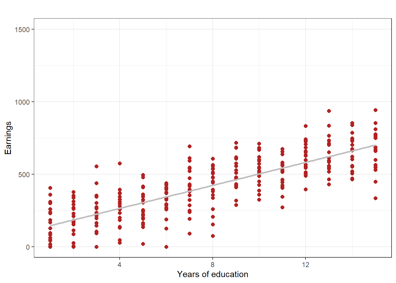
Figure 4.2: Illustration of homoskedasticity, using simulated data
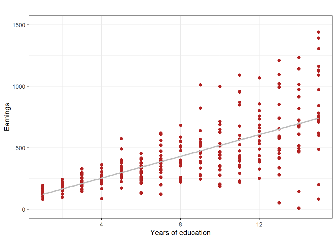
Figure 4.3: Illustration of heteroskedasticity, using simulated data
After this digression, we return to our problem. For many decades, researchers could calculate the standard error of the regression coefficient under the assumption of homoskedasticity. But there was no consensus about how to calculate the standard error of an estimated coefficient if there was heteroskedasticity.
If the errors \(\epsilon_i\) were homoskedastic, that is, if the variance of the errors did not depend on the level of \(X\), the formula was straightforward. Mathematically, using the conditional expectations operator, the assumption of homoskedasticity is that \(E(\epsilon_i^2|X_i)=E(\epsilon_i^2)\) for each \(i = 1, ...,N\). In this case, the formula for the variance of the estimator for \(\beta_1\) is given by:
\[SE\hat{\beta_1})^{homoskedasticity} = \sqrt{\frac{\frac{1}{n-2}\sum\nolimits_{i=1}^{N}\epsilon_i^2}{\sum\nolimits_{i=1}^{n}(x_i - \overline{x})^2}}\] The assumption of homoskedasticity is quite unreasonable. Suppose one were estimating the relationship between years of education and wages. At low levels of education (around high school levels) most workers earn low wages, and the variance of wages is small around the mean wage. At high levels of education, beyond university level, earnings might be very variable. The errors around the mean earnings, then, are heteroskedastic conditional on education levels. The assumption of homoskedasticity persisted, however, because no statisticians could figure out how to calculate the standard errors for a regression coefficients if the errors were heteroskedastic.
If the variance of the error does depend on the level of \(X\), the errors are heteroskedastic. It took about 50 years after the introduction of regression analysis for researchers to figure out the formula to calculate the “correct” standard errors. These are sometimes called robust standard errors, or Eicker–Huber–White standard errors after the researchers who share credit with determining the formula (Eicker, 1967; Huber, 1967; White, 1980). The formula takes into account heteroskedasticity (that the distribution of errors may vary with the level of \(X\)). The estimator for the correct standard error of the OLS estimator of the slope coefficient in the single variable regression is: \[SE(\hat{\beta_1})^{heteroskedasticity} = \sqrt{\frac{1}{n} * \frac{\frac{1}{n-2} \sum\nolimits_{i=1}^n (x_i - \overline{x})^2 \hat{\epsilon}_i^2}{[\frac{1}{n}\sum\nolimits_{i=1}^n (x_i - \overline{x})^2]^2}}\] Whichever formula is used, it can be seen that the standard error is smaller if the regression fits better (so that the standard error of the regression (SER or RMSE) is smaller), and if the sample size is larger.
Even at the time of writing this book, 2024, many software packages, including R, calculate standard errors using a formula that assumes the error are homoskedastic. In displaying regression results, one has to be proactive and use various options in the commands to generate corrected standard errors.
4.3.2 Hypothesis test with estimated coefficient
We are now ready to return to the initial problem of making more precise what we mean by the question of how much confidence we should have in the estimated coefficient. One approach to make this question more precise is to follow a tradition in the social science of carrying out a hypothesis test. That is, we assume a null hypothesis (“I think the following is true about the population”) and ask whether what we calculate from a sample of data from the population is consistent with that hypothesis. More specifically, we calculate what the probability is that, if the null hypothesis were indeed true, we would observe a value for the estimator of the coefficient \(\beta_1\) as different from the null hypothesis as that which we observe. “As different” is sometimes phrased as “as far away or more far away from the null hypothesis.” If the probability of calculating a number comparable (in terms of the hypothesis) to the number we actually calculate (the coefficient) is high, then we continue to accept our null hypothesis. If the probability of calculating the number we actually calculate, or even further away numbers, is sufficiently low, then we reject the null hypothesis.
The wording can seem forced here. Remember that the probability of calculating any particular coefficient is essentially zero, for a continuous variable. Since the estimated coefficients can have many decimal places, the probability of calculating 5.673027 as a coefficient is essentially zero. So that is not the probability calculation we have in mind. Instead we think more along the lines of: what is the probability of estimating a coefficient that is so inimical to my null hypothesis that I would reject the null hypothesis? If the null hypothesis is that the coefficient of the slope is 0, how big would my estimated coefficient have to be, in absolute value, for me to reject the null hypothesis? That probability is not a point probability, but rather a range: the probability of calculating an estimated coefficient that big or bigger… if the “big” coefficient in absolute value leads me to reject the null hypothesis, then even bigger coefficients would also.
What is a “sufficiently low” probability? By convention in the social sciences this is 5%. If the probability is less than 5% then we reject. This threshold or standard is arbitrary, and partly depends on the consequences of accepting or rejecting the null hypothesis. In many social sciences, the consequences of research are small: the typical social science research, whether published or unpublished, is not read by people outside of the social science community. Occasionally, though, social science research can be very influential. In the COVID-19 pandemic, for example, many substantial policy decisions were made by government elected officials, and disputes of the constitutionality of policies were decided by judges, where empirical evidence and the conclusions of social scientists mattered. This hypothesis testing approach is somewhat like the way evidence is used in legal disputes, where traditions speak of a “preponderance” of evidence or evidence leading to a conclusion “beyond the shadow of a doubt.” In legal cases, one is either guilty or not guilty, and the legal system cannot find a person “possibly guilty with probability of 27%.”
Another influential way of thinking about assessing the confidence one might have in the results of econometric analysis is to suppose that stakeholders have a prior belief about the true value of the parameter. With each new study they read, they update their beliefs. The more credible a study, the more they might update if the new estimate differs from their prior estimate. The less credible a study, the less they might update. The approach is sometimes referred to as the Bayesian approach (Lancaster, 2004). We shall stick to the hypothesis testing framework in this book.
To implement the hypothesis test, we need three numbers: the null hypothesis of the value of the coefficient, the estimate of the coefficient, and the standard error of the estimated coefficient. We use these to calculate a test statistic, often called a t-statistic, or t-stat for short. \[t-statistic = \frac{estimate - hypothesizedvalue}{standard error of estimate} = \frac{\hat{\beta_1} - \beta_1^{null}}{SE(\hat{\beta_1})}\] The null hypothesis about regression coefficients, by convention in most of the social sciences, is that the coefficient is equal to 0. That is, the null hypothesis is that the explanatory variable has no effect on the outcome, or does not influence the outcome. Other null hypotheses are possible: that the coefficient is positive; that the coefficient is negative; that the coefficient is greater than some value. Testing these other hypotheses is a straightforward extension of the basic hypothesis test. In the conventional hypothesis test, \(\beta_1^null = 0\), so we have, \[ t-statistic = \frac{\hat{\beta_1} - 0}{SE(\hat{\beta_1})} = \frac{\hat{\beta_1}}{SE(\hat{\beta_1})}\] The t-statistic is the estimated coefficient divided by the estimated standard error of the coefficient.
The Central Limit Theorem in probability and statistics theory can be used to show that if the sample size is reasonably large, the t-statistic follows the standard normal distribution. The normal distribution is characterized by the mean \(\mu\) and standard deviation \(\sigma\) and is written as \(N(\mu, \sigma^2)\). The density function of the normal distribution for a variable x is, \[ f(x) = \frac{1}{\sqrt{2\pi}\sigma}e^{-(x-\mu)^2/(2\sigma^2)}\] The standard normal distribution has mean equal to zero and standard deviation equal to one, so it is \(N(0, 1)\). The cumulative distribution of the standard normal distribution is written as, \[P(x \le c) = \Phi(c) = \int_{\infty}^c \frac{1}{\sqrt{2\pi}}e^{-x^2/2}, x \sim N(0,1)\] This is the probability of obtaining a value of the random variable \(x\) that is less that the value \(c\).
Since the t-statistic follows the standard normal distribution, the probability (called the p-value) of obtaining an actual estimate of the coefficient as far away from the null hypothesis (zero) as one obtains with the sample is given by, \[p-value = P(x \le - |t-stat|) + P(x \ge |t-stat|) = 2 * \Phi(-|t-stat|)\] where the second equality follows because the normal distribution is symmetric. The expression \(|t-stat|\) is the absolute value of the t-statistic. That is, this is the probability of falling far away in the left tail, and falling far away in the right tail, where “far away” is defined by the absolute value of the t-stat, which is the coefficient divided by the standard error.
A numerical example may help. Suppose the estimated coefficient in a single variable regression is 2.6 and the standard error is 1.3. Then the tstatistic is 2.00. The probability of observing a t-statistic at least as far away from zero as 2 is, is given by,
\[p-value = P(x \le -|2|) + P(x \ge |2|) = 2 * \Phi(-|2|)\]
The interesting thing about the normal distribution is that even before computers, human “computers” had calculated to several decimal places the cumulative probability distribution. These probabilities were reprinted in tables in every statistics and econometrics book; see for example Figure 3. When computers because ubiquitous, an individual could simply look up the value in many software packages. Even the Excel spreadsheet software can automatically compute the cumulative probability.

In statistical computing software such as R, one uses the command pnorm(c)
to calculate the cumulative probability of the standard normal distribution
at a certain value c. So we find that pnorm(-|2|) equals 0.02275013. We
want 2*pnorm(-|2|), so that is approximately .045. The probability, then,
of obtaining an estimated regression coefficient of 2.6 and a standard error
of 1.3 is only 4.5% if the null hypothesis is true, so since this is lower than
the conventional 5% threshold, we reject the null hypothesis.
4.3.3 Some intuition about the p-value
To recap, the p-value is the probability of calculating, under the assumption that the null hypothesis is true, and with a sample of data from the population, a coefficient \(\hat{\beta_1}\) at least as different (as far away) from the null hypothesis \(\beta_1^{null}\) as the coefficient that we actually calculated (\(\hat{\beta_1}^{actual}\)). Sadly, there is no other way to say that in a more intuitive manner. It is a complex expression. That is why econometrics is hard.
Notice that the p-value depends on the t-statistic, which has \(SE(\hat{\beta_1})\) in the denominator. The standard error of the estimated coefficient depends, in turn, on three values: the sample size \(n\), the variation in \(X\), as measured by \(\sum\nolimits_{i=1}^n (x_i - \overline{x})^2\), and a more complex term that for intuitive purposes we can call the size of the estimated squared residuals, weighted by the \(X\) value associated with each residual deviation from the mean, \(\sum\nolimits_{i=1}^n (x_i - \overline{x})^2\hat{\epsilon}_1^2\). If the sample size is larger, the standard error will be smaller. If the variation in \(X\) if larger, the standard error will be smaller. If the squared residuals are smaller, the standard error will be smaller. The standard error determines the denominator of the t-statistic, which determines the p-value, which determines our sense of how much confidence to have that the estimated coefficient is different from zero (i.e., should we reject the null hypothesis that there is no relationship). If the sample size is large, and there is a lot of variation in the explanatory variable, and the regression line fits the data well (the residuals are small), then we have more confidence in the value of our estimated coefficient (and it being different from zero). If, on the other hand, the sample size is small, and the explanatory variable has little variation, and the regression line does not fit the data well (the residuals are large), then we have little confidence in our coefficient, and would not reject the null hypothesis that the coefficient is zero.
One other observation to make is that in hypothesis testing of coefficients, it is common to use a shorthand phrase, “the coefficient is statistically significant” to mean that the null hypothesis of the coefficient being equal to zero is rejected.
4.3.4 Confidence interval of estimated coefficient
If the wording for explaining what the p-value struck you, dear reader, as complex, wait until you see the convoluted wording for explaining what a confidence interval for an estimated coefficient is. Even experienced social scientists resort to ad hoc intuitive sounding explanations that are not quite right, and they get “called out” for their imprecision. Let us simply quote several master econometricians, who put forth several equivalent ways to express the idea precisely (Stock and Watson, 2015; Wooldridge, 2015): • “A confidence interval for \(\hat{\beta}_1\) is the set of values that cannot be rejected using a two-sided hypothesis test with a 5% significance level.” • “A confidence interval for \(\hat{\beta}_1\) is an interval that has a 95% probability of containing the true value of \(\beta_1\); that is, in 95% of possible samples that might be drawn, the confidence interval will contain the true value of \(\beta_1\).” • “The proper way to consider the confidence interval is that if we construct a large number of random samples from the population, 95% of them will contain \(\beta_1\): Thus, if a hypothesized value for \(\beta_1\) lies outside the confidence interval for a single sample, that would occur by chance only 5% of the time.”
In practice, the calculation of the confidence interval for a regression coefficient is remarkably simple. \[CI_{95\% level} =[\hat{\beta}_1 - 1.96 * SE(\hat{\beta}_1), \hat{\beta}_1 + 1.96 * SE(\hat{\beta}_1) ]\] Where does the number 1.96 come from? For a variable that follows the standard normal distribution, the probability of obtaining outcomes greater than 1.96 is 2.5%, and the probability of obtaining outcomes less than -1.96 is 2.5% (by symmetry), so the probability of an outcome as far away from 0 (or more) in absolute value as 1.96 is from 0, is 5%.
4.4 Using R to calculate regression results
Let us turn to R to examine regression output that includes hypotheses
tests and confidence intervals. First, in a blank script, we copy and paste the
usual preliminaries, from our earlier script. We clear the working environment
with the code rm(list = ls()), load packages, and run other settings,
Then we read in the Kenya, as in the previous chapter, with the following
code:
# Read Kenya DHS 2022 data from a website
url <- "https://github.com/mkevane/econ42/raw/main/kenya_earnings.csv"
kenya <- read.csv(url)
We then have R run the regression withe following command. The results
are stored in the object reg1, and command summary(reg1) displays the
regression results.
# Calculate regression coefficient and residuals
reg1 <- lm(earnings_usd ~educ_yrs, data=kenya)
summary(reg1)
Call:
lm(formula = earnings_usd ~ educ_yrs, data = kenya)

Residuals:
   Min     1Q Median     3Q    Max
  -861   -248   -118     85  41206

Coefficients:
            Estimate Std. Error t value Pr(>|t|)
(Intercept)  -175.87      13.85   -12.7   <2e-16 ***
educ_yrs       51.89       1.31    39.8   <2e-16 ***
---
Signif. codes:  0 '***' 0.001 '**' 0.01 '*' 0.05 '.' 0.1 ' ' 1

Residual standard error: 787 on 22084 degrees of freedom
Multiple R-squared:  0.0668,    Adjusted R-squared:  0.0668
F-statistic: 1.58e+03 on 1 and 22084 DF,  p-value: <2e-16
The object reg1 appears in your workspace environment (upper right).
Note that the command lm(...) is the linear model (regression) function.
The first variable is the \(Y\) variable, then any \(X\) variable(s) are included
after the ∼. The \(X\) variable, here \(educ\_yrs\), is the explanatory variable or
the regressor. We gave the regression output a name, reg1. Notice data=df
in the lm command. This allows us to just use the variable names in this
function without including the data set name and $ sign. To see the actual
results of the regression in your console, highlight and run the summary(...)
command. In the future, we will not do this, but let us take a look. Here is
the relevant part of the regression output in your console:
##
## Call:
## lm(formula = earnings_usd ~ educ_yrs, data = kenya)
##
## Residuals:
##    Min     1Q Median     3Q    Max
##   -861   -248   -118     85  41206
##
## Coefficients:
##             Estimate Std. Error t value Pr(>|t|)
## (Intercept)  -175.87      13.85   -12.7   <2e-16 ***
## educ_yrs       51.89       1.31    39.8   <2e-16 ***
## ---
## Signif. codes:  0 '***' 0.001 '**' 0.01 '*' 0.05 '.' 0.1 ' ' 1
##
## Residual standard error: 787 on 22084 degrees of freedom
## Multiple R-squared:  0.0668, Adjusted R-squared:  0.0668
## F-statistic: 1.58e+03 on 1 and 22084 DF,  p-value: <2e-16
Note that the implied regression equation is: \(earnings usd = −23+15 ∗
educ\_yrs\). The intercept is 30.177 and the slope is 19.914. Plainly, there
is no need for so many decimal places; we could just as well say the slope
coefficient is about 20. The p-value of the hypothesis test for the coefficient
on education is given by Pr(>|t|). It is very small (less than 2e-16, which is
.00000000000000002), clearly less than .05, so we reject the null hypothesis
of no relationship. We might say “the coefficient on the education variable
is statistically significant.”
4.4.1 Create a table of regression results with corrected standard errors
Economists usually present regression results in a different format. The
coefficients from a regression are presented in the form of a table, with each
column the results of one regression. This way, a table might consist of
five columns, each one the result of a different regression. We can use the
modelsummary command in the modelsummary package to make very nice
regression tables. In addition, we want to use the corrected standard errors
for the coefficients. Let us make the table and see what we get. Copy and
paste the next block of code into R and run the code.
modelsummary(reg1,
fmt = fmt_decimal(digits = 3, pdigits = 3),
stars=T,
vcov = 'robust',
gof_omit = "IC|Adj|F|Log|std",
title = 'How much does education affect earnings?')| (1) | |
|---|---|
| (Intercept) | −175.872*** |
| (15.447) | |
| educ_yrs | 51.895*** |
| (1.992) | |
| Num.Obs. | 22086 |
| R2 | 0.067 |
| RMSE | 786.60 |
| Std.Errors | HC3 |
| + p < 0.1, * p < 0.05, ** p < 0.01, *** p < 0.001 |
Notice that everything within the set of parentheses following the command
modelsummary is part of the same command. Within the parentheses,
note:
• reg1 is the name of the regression; more generally we would have a list
of regressions to display.
• vcov = ’robust’ is how we tell R to use the corrected standard errors.
If you omitted this option, modelsummary would just use the uncorrected
SEs. In many statistical packages (including R), the default
regression function calculates coefficient standard errors that are only
valid if the error term is homoscedastic. That is, the variance of the
error (unexplained part) is the same for all observations. There is no
reason to think this would be true, and if it is not, the standard errors
are incorrect, and so are the resulting hypothesis tests. To fix this, we
include in the modelsummary command the option vcov = ‘robust’.
This option tells R to recalculate the standard errors to be consistent
with heteroskedasticity.
• title=… gives the table a title. Put the title in quotes.
• gof_omit = "IC|Adj|F|Log|std" means the table of regression output
will omit some summary statistics of goodness of fit (gof) that
are the default. For our purposes we usually only want the R-Square
statistic and the RMSE or SER. Always use this option.
• digits=3 rounds the numbers in the table to three digits after the decimal.
You can change this if you like.
Now highlight and run the modelsummary command (all lines of it…make sure you include all parentheses!). If you get an error message, most
likely you have not loaded the modelsummary package with the command
(library(modelsummary)). Also recall that if you highlight and run just
part of a command, and it includes an open parenthesis, then R will be
waiting for the close parenthesis, and will not give any output. You might
see a plus sign (+) in the Console window. Click down there and hit the Esc
key. See the earlier chapter for how to resolve this problem.
Examine the results in the viewer frame (lower right) in RStudio, which
are reproduced in Table 1.
| (1) | |
|---|---|
| (Intercept) | −175.872*** |
| (15.447) | |
| educ_yrs | 51.895*** |
| (1.992) | |
| Num.Obs. | 22086 |
| R2 | 0.067 |
| RMSE | 786.60 |
| Std.Errors | HC3 |
| + p < 0.1, * p < 0.05, ** p < 0.01, *** p < 0.001 |
The slope and intercept coefficient estimates, with standard errors in parentheses. The significance codes (asterisks) are for the null hypothesis that the coefficient is zero. *** means the p-value is between 0 and 0.01, so the null can be rejected at the 0.01 = 1% level. The coefficient called “Intercept” is the estimate of the Y intercept, or constant.
“Num. Obs.” is the number of observations used in the estimation. “R2” gives the \(R^2\) measure of goodness of fit of the regression. “RMSE” is another label for the standard error of the regression (SER), also known as the Residual Standard Error. The “Std. Errors” as “HC3” indicates that modelsummary uses a particular way to calculate the heteroskedasticadjusted standard errors for the coefficients.
You can compare these results with the table of regression results without
the robustness correction. Simply run the code below, which is the same as
the earlier code chunk but without the option vcov = ’robust’.
modelsummary(reg1,
fmt = fmt_decimal(digits = 3, pdigits = 3),
stars=T,
gof_omit = "IC|Adj|F|Log|std",
title = 'How much does education affect earnings?')| (1) | |
|---|---|
| (Intercept) | −175.872*** |
| (13.851) | |
| educ_yrs | 51.895*** |
| (1.305) | |
| Num.Obs. | 22086 |
| R2 | 0.067 |
| RMSE | 786.60 |
| + p < 0.1, * p < 0.05, ** p < 0.01, *** p < 0.001 |
Note that the point estimates are the same (e.g., the slope is 19.9), whereas the standard errors are slightly different. With this data sample, the standard errors for the slope coefficient in the first case are slightly larger due to the correction for heteroscedasticity. The correction seldom makes a large difference, but it is good practice. Hence, we will always use a correction of the standard errors.
4.4.2 Retrieve and plot the regression residuals
The regression residuals are the difference between the actual value of the dependent variable (Y) and the predicted value from the regression, for each observation. A scatterplot of the residuals can provide a useful diagnostic of the appropriateness of the regression. Highlight and run the following commands:
kenya$resid1 = kenya$earnings_usd - (reg1$coefficients[1] +
reg1$coefficients[2]*kenya$educ_yrs)
ggplot(data=subset(kenya,earnings_usd<=1000), aes(x=educ_yrs, y=resid1)) +
geom_point(size = 2, col = "firebrick", shape = 16)+
labs(x="Years of education",
y="Regression residual")+
theme_bw()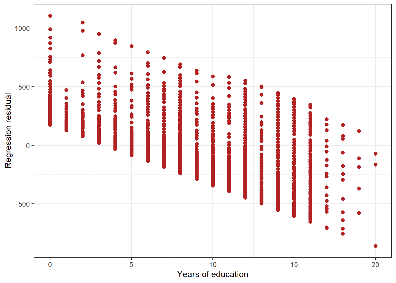
Figure 4.4: Figure 4: Residuals associated with different levels of education
Do you see any pattern in the plot, reproduced as Figure 4? It seems that the residuals gradually decrease in size for individuals with higher levels of education. We shall see in later chapters that this potentially indicates misspecification of the model. Perhaps the relationship is not actually linear, as assumed here.
4.5 Recapitulation, in the style of Cormac McCarthy
As usual, we asked ChatGPT to generate text that summarizes some key ideas of this chapter. Here is the text generated:
In the austere realm where numbers converge with a silent determination, the method known as Ordinary Least Squares casts its unyielding shadow. Here, amidst the relentless pursuit of truth amidst uncertainty, stand the four foundational assumptions, each akin to the unbroken earth beneath a solitary traveler’s weary tread.
First among these, as immutable as the passage of celestial bodies across a starlit sky, is the assumption of linearity. It commands that the relationship between the dependent variable and its covariates shall be as straight and unwavering as the path of a lone rider through the vast expanse. This linearity, unseen yet foundational, bestows upon regression its form and purpose, guiding the seeker toward understanding. Second, like the echoing silence of untouched wilderness at dusk, comes the assumption ofindependence and identically distributed errors (i.i.d.). Each observation, a solitary beacon in the twilight of data’s vast expanse, must stand free from the influence of its kin. This independence ensures that the errors, those elusive echoes of truth, are neither constrained nor colored by the destiny of their predecessors, allowing the essence of each observation to speak for itself. Third, akin to the unbroken horizon stretching to infinity, lies the assumption of no correlation between the errors and the independent variables (X). It commands that the capricious whims of error shall not bow to the subtle nudges of covariates, preserving the sanctity of their distinction. This absence of correlation ensures that the measured impact of each covariate remains steadfast and true, unswayed by the whispers of uncertainty. And fourth, like the vigilance of a lone sentinel in the wilderness, stands the assumption of a low probability of outliers. It declares that within the vast expanse of data’s frontier, anomalies shall hold little sway. This vigilant watch over the outliers, those rogue elements seeking to disrupt the harmony of analysis, secures the integrity of regression’s measured stride, allowing truth to emerge from the quietude of normalcy.
Thus, within these four sacred tenets lies the covenant of Ordinary Least Squares, forging a path where numbers speak with the stark clarity. In this unyielding landscape of statistical inquiry, these assumptions stand resolute, guiding the seeker toward the elusive horizon where certainty and truth converge.
Words, it seems to us, worthy of being etched in marble.
Review terms and concepts: • inference • random variable • probability distribution • standard normal distribution • expected value • conditional expectation • hypothesis test • null hypothesis • t-statistic • p-value • confidence interval • residuals
References Anscombe, Francis J (1973). “Graphs in statistical analysis”. In: The american statistician 27(1). Publisher: Taylor & Francis, pp. 17–21. Eicker, Friedhelm (1967). “Limit theorems for regressions with unequal and dependent errors”. In: Proceedings of the Fifth Berkeley Symposium on Mathematical Statistics and Probability, Volume 1: Statistics. University of California Press, pp. 59–82. Huber, PJ (1967). “The behavior of maximum likelihood estimates under nonstandard conditions”. In: Proceedings of the Fifth Berkeley Symposium on Mathematical Statistics and Probability, Volume 1: Statistics. University of California Press, pp. 221–233. Lancaster, Tony (2004). An introduction to modern Bayesian econometrics. Blackwell Oxford. Stock, James H and Mark W Watson (2015). Introduction to Econometrics 3rd ed. Pearson Education. White, Halbert (1980). “A heteroskedasticity-consistent covariance matrix estimator and a direct test for heteroskedasticity”. In: Econometrica: journal of the Econometric Society. Publisher: JSTOR, pp. 817–838. Wooldridge, JeffreyM(2015). Introductory econometrics: A modern approach. Cengage learning.