6 Log Specifications
Abstract
This chapter covers nonlinear regression specifications that use log-transformed variables.
Keywords: Log specifications, regression
6.1 Introduction: Capturing nonlinear relationships
Up to now we have considered regressions that are modeled as linear functions between two variables: \(Y = β_0 + β_1X\). The linear probability model, seen in the previous chapter, is somewhat more complex, but has a straightforward interpretation. But there is no reason to expect all relationships between variables to resemble straight lines, and econometrics has various ways to estimate regression models that allow for nonlinear relationships. We will consider several of these, and in this chapter we explore one of the most important and widely used of these methods: namely, log-transformed variables. Basically, we use the natural logarithm (log) of a variable in the regression, rather than the variable itself. Doing this has a number of desirable properties. Most importantly, in many circumstances it transforms a non-linear relationship into a linear relationship that can be estimated using OLS. Before we explain this feature, let’s refresh your memory about the natural log function.
6.2 The natural log function
The logarithmic function with natural number e as base is one of those mysterious mathematical relationships that some people refuse to learn. But no reader of this book shares the anxiety that rejects understanding, amirite? Consider the number e represented by 2.71828 . . . . Like π, e is an irrational number. It cannot be represented as a ratio of integers. As an irrational number, the decimals go on infinitely and do not repeat, but that does not mean we cannot consider it to be a number. (Believe it or not, many people of the generation of the authors were taught that \(π = \frac{22}{7}\) which is close but not exactly right. They lied to us, thinking they were doing us a favor.)
The number e is a very useful number. For one thing, it is the limit of \((1+
1/n)^n\) as n approaches infinity. It is a key part of the formula for calculating
compound interest, and thus essential in modern finance. Knowing a bit
about e, we can define the natural logarithm (or just “log”) of a number \(x\)
as the power to which e would have to be raised to equal \(x\). Thus the log
is the inverse function of (“undoes”) the exponential function, \(y = log(x) ⇒ x = ey\). For example, \(log(5) = 1.6094...\), because \(e^{1.6094...} = 5\). Note that the natural logarithmic function is sometimes written as ln() and sometimes as
log(). Because the natural log operator in R is log(X), we will use log() in
this text to avoid confusion. There are also logarithmic functions with bases
other than e, such as \(log_{10}(X)\) (base 10), but these other bases are rarely
used in econometrics.
6.2.1 Use R to visualize the log function
To see what the log function looks like, use R to draw the curve:
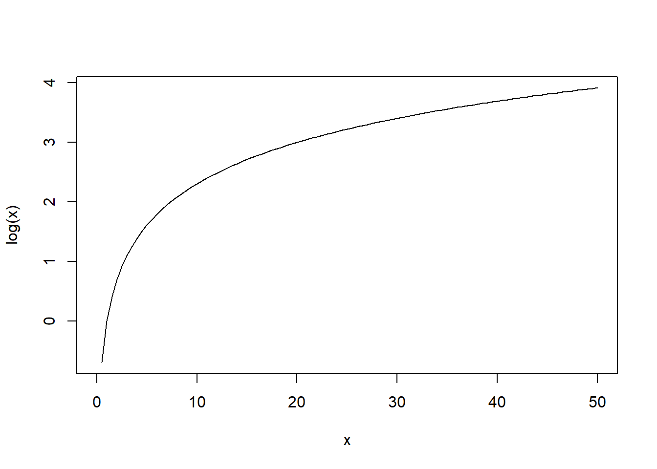
You can easily see this is a non-linear relationship.
We can use R to see how the log function can transform a non-linear relationship into a linear relationship. Draw the following two curves in R.
curve(exp(.7*x), n=50,from=0, to=5, col="red",
xlab="X - explanatory variable", ylab="Y - outcome")
curve(log(exp(.7*x)), from=0, to=5, add=TRUE, col="blue")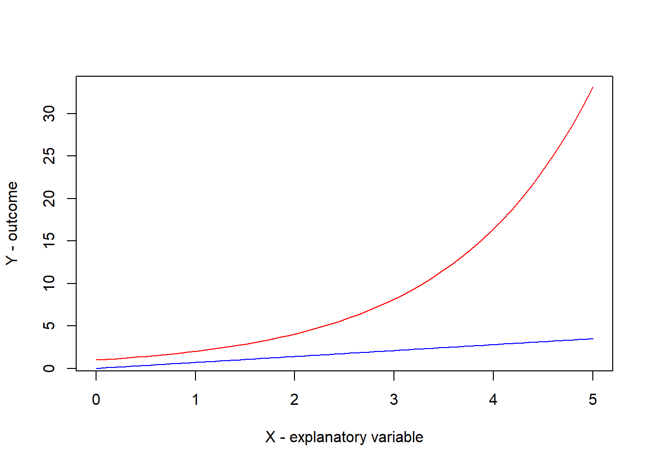
Notice that for the second curve we have the value of \(Y\) in the first curve, which is \(e^{.7X}\), transformed by the log function. And so the second relationship between \(X\) and this transformed \(Y\) is a straight line, with slope .7.
6.2.2 Some useful properties of logs
The most important mathematical property of logs for our purposes is that the log function acts as a “proportionalizer”: For small changes, the change in the log of a variable is approximately equal to the proportional change in the variable itself (or, multiplying by 100, the percentage change).This property is precisely true for infinitesimal changes, because the derivative of the log function is \(1/X\), and thus: \[\mathrm{d}log(X)=\frac{\mathrm{d}X}{X}\]
The expression \(dX/X\) is simply the proportional change in \(X\). For larger but still fairly small changes in \(X\), this relationship is not exact but is still approximately true. So it is quite common in economics to think of changes in log variables as approximate proportional changes. For example, consider a change in \(X\) from 1.00 to 1.05, which we would consider a proportional increase of \((1.05 - 1.00)/1.00 = 0.05 = 5\%\). Taking logs, \(Δlog(X) = log(1.05) − log(1.00) = 0.0488 ≈ 0.05 = 5\%\).
A nice property of the change in logs is that it is symmetrical for increases and decreases: the change from 1.05 back down to 1.00 starting from the base of 1.05 would be \(Δlog(X) = log(1.00) − log(1.05) = −0.0488\). Furthermore, the change in logs lies between the proportional changes that would be calculated using the start vs. end values as the base of comparison:
\[\frac{1.05-1.00}{1.05} = 0.0476 < \Delta log(X) = 0.0488 < \frac{1.05-1.00}{1.00} = 0.0500\] Some additional properties of the log function that we use are the following:
\[log(e) = 1\] \[log(1) = 0\] \[log(0) = \text{undefined, cannot take log of zero}\] \[log(−|x|) = \text{undefined, cannot take log of negative number}\] \[log(1/x) = −log(x)\] \[log(ax) = log(a) + log(x)\] \[log(a/x) = log(a) − log(x)\] \[log(xa) = alog(x)\] ### Three specifications using the log function
In terms of empirical models about economic relationships, there are three specifications that use the log transformation of a variable. The three specifications are usually called the log-linear, log-log, and linear-log specifications.
Probably the most common is the log-linear specification. The outcome variable is logged, but the \(X\) variable is not.
\[log(Y) = β_0 + β_1X\] We interpret the slope \(β_1\) as (for small changes in \(X\): \[\beta_1 = \frac{\mathrm{d}log(Y)}{\mathrm{d}X} = \frac{\text{proportional change in Y}}{\text{change in X}}\] Another common specification is the log-log specification. Both the outcome and the explanatory variable are logged. That is, we log-transform both the dependent variable and the regressor. \[log(Y ) = β_0 + β_1log(X)\]
We interpret the coefficient as the proportional change in \(Y\) for a proportional change in \(X\). \[\beta_1 = \frac{\mathrm{d}log(Y)}{\mathrm{d}log(X)} = \frac{\text{proportional change in Y}}{\text{proportional change in X}}\] Equivalently, and more commonly, we interpret the coefficient as the elasticity: the proportional (percent) change in \(Y\) for a proportional (percent) change in \(X\). \[\beta_1 = \frac{\mathrm{d}log(Y)}{\mathrm{d}log(X)} * \frac{100}{100} = \frac{\text{percent change in Y}}{\text{percent change in X}}\] Students of economics might find that this formula rings a bell somewhere deep in their econ-brain; it defines the price elasticity of demand or of supply. For example, if we have data that describes a demand relationship between the price charged for a good \(P\) and the quantity that people buy \(Q\), the price elasticity of demand would be
\[η_D = elasticity = \frac{\text{proportional change in Q demanded}}{\text{proportional change in P}}\]
Given data on prices and quantities demanded for a good, we could estimate the elasticity of demand directly using a log-log specification:
\[log(Q) = \beta_0 + η_Dlog(P)\]
For example, if the estimated slope \(ηD\) turned out to be equal to -2.0, this would imply a demand elasticity of -2, which is relatively elastic: For a 1% increase in price, quantity demanded would decrease by 2%.
Although log-log regressions have this potentially useful interpretation, care must be taken in estimating elasticities. The biggest problem is that in real-world data, the observed combinations of P and Q are usually a result of the interaction of both demand and supply relationships, as students of microeconomics will recall. Consequently, in practice, the regression is estimating neither a demand elasticity nor a supply elasticity, but some complex combination of the two.
A less common specification is the linear-log specification. The explanatory variable is logged. \[Y = β_0 + β_1log(X) (10)\] We interpret the slope \(β_1\) as (for small changes in \(X\) the unit change in Y for a proportional change (or percentage change) in \(X\). \[\beta_1 = \frac{\mathrm{d}Y}{\mathrm{d}log(X)} = \frac{\text{change in Y}}{\text{proportional change in X}}\] Box 6.1 develops some of the algebra to demonstrate these intuitions about how to interpret coefficients estimated in log specifications.
Box 6.1: Algebra and calculus demonstration of how to interpret coefficients in log specifications
In order to understand better how to interpret the coefficients in these specifications, we use the result that \(ln(1+\Delta) \thickapprox \Delta\) when \(\Delta\) is a small number, such as .05 or .01 (in R, run the commands and , or, better yet, plot the difference and see how it gets very small as \(x\) gets smaller. This code should do that: .
Now, let us consider the log-log specification. Let \(\Delta\) represent a small percent change (we use the decimal version rather than a % version, so \(\Delta\)=.01 represents a 1% change and \(\Delta\)=1 represents a 100% change. We have then equations for the outcomes \(Y\) and \(Y^{new}\), \[\begin{align*} ln(Y) &= \beta_0 + \beta_1 ln(X) \\ ln(Y^{new}) &= \beta_0 + \beta_1 ln(X(1+\Delta)) \end{align*}\] We are interested in determining how much \(Y\) changes when \(X\) changes by \(\Delta\). That is, we want to know \(Y^{new}-Y\). We note that we can use the rules of logarithms to rewrite, \[\begin{align*} ln(Y^{new}) &= \beta_0 + \beta_1 ln(X) + \beta_1 ln(1+\Delta)) \\ ln(Y^{new}) &= \beta_0 + \beta_1 ln(X) + \beta_1 \Delta \end{align*}\] Then we can subtract the old value of \(Y\) from the new value of \(Y\), \[\begin{align*} ln(Y^{new})-ln(Y) &= \beta_0 + \beta_1 ln(X) + \beta_1 \Delta -[\beta_0 + \beta_1 ln(X)]\\ ln(Y^{new})-ln(Y) &= \beta_1 \Delta \end{align*}\] Using another rule of logarithms, and then judicious adding and subtracting, and then our small change result from above, we rewrite, \[\begin{align*} ln(Y^{new}/Y) &= \beta_1 \Delta \\ ln(Y/Y + (Y^{new}-Y)/Y) &= \beta_1 \Delta \\ ln(1 + (Y^{new}-Y)/Y) &= \beta_1 \Delta\\ (Y^{new}-Y)/Y &\thickapprox \beta_1 \Delta \\ \beta_1 &\thickapprox \frac{(Y^{new}-Y)/Y}{\Delta} \\ \beta_1 &\thickapprox \frac{(Y^{new}-Y)/Y}{\Delta} \frac{100}{100} \\ \beta_1 &\thickapprox \frac{\mbox{percent change in Y}}{\mbox{percent change in X}} \end{align*}\]
If our specification is a log-log specification, we interpret the coefficient as the percent change in \(Y\) resulting from a 1% change in \(X\).
Now, let us consider the log-linear specification. Again, let \(\Delta X\) represent a small unit change in \(X\) and \(\Delta Y\) represent a small unit change in \(Y\). We have then equations for the outcomes \(Y\) and \(Y^{new}\), \[\begin{align*} ln(Y) &= \beta_0 + \beta_1 X \\ ln(Y^{new})= ln(Y + \Delta Y) &= \beta_0 + \beta_1 (X+ \Delta X) \end{align*}\] So then, \[\begin{align*} ln(Y + \Delta Y)-ln(Y) &= \beta_1 \Delta X \end{align*}\] and then, \[\begin{align*} ln(\frac{Y + \Delta Y}{Y}) &= \beta_1 \Delta X \\ ln(1 + \frac{\Delta Y}{Y}) &= \beta_1 \Delta X \\ \frac{\Delta Y}{Y} &\thickapprox \beta_1 \Delta X \\ \beta_1 &\thickapprox \frac{\Delta Y/Y}{\Delta X } \\ \beta_1 * 100 &\thickapprox \frac{\Delta Y/Y}{\Delta X } * 100 \\ \beta_1 * 100 &\thickapprox \frac{\mbox{percent change in Y}}{\mbox{1 unit change in X}} \end{align*}\] If our specification is a log-linear specification, we multiply the coefficient by 100 and then interpret that number as the percent change in \(Y\) resulting from a 1 unit change in \(X\). That is, we multiple the estimated coefficient \(\beta_1\) by 100, and consider that to be the percent change in \(Y\) for a 1 unit change in \(X\).
Note that if we use calculus and take the total derivative of the equality, we can quickly arrive at a similar interpretation: \[\begin{align*} \frac{d ln(Y)}{d Y} &= \frac{ d(\beta_0 + \beta_1 X)}{d X} \\ \frac{1}{Y} dY = \frac{dY}{Y} = \frac{Y^{new}-Y^{old}}{Y^{old}} &= \beta_1 dX \\ \beta_1 &=\frac{\frac{Y^{new}-Y^{old}}{Y^{old}} }{ dX} \\ 100* \beta_1 &=\frac{100*\frac{Y^{new}-Y^{old}}{Y^{old}} }{ dX} \\ 100* \beta_1 &=\frac{\mbox{percent change in Y} }{ \mbox{ unit change in X} } \end{align*}\]
Consider the final case, the linear-log specification. We can use calculus and take the total derivative of the linear-log specification, with GDP per capita as the outcome and a measure of overall average education attainment in countries as the explanatory variable: \[\begin{align*} d GDP &= \frac{ d(\beta_0 + \beta_1 ln(EDUC)}{d EDUC} \\ d GDP &= \beta_1 \frac{EDUC^{new}-EDUC^{old}}{EDUC^{old}} \\ d GDP &= \frac{\beta_1}{100} \frac{100*(EDUC^{new}-EDUC^{old})}{EDUC^{old}} \\ \frac{\beta_1}{100} &= \frac{\mbox{unit change in GDP}} {\mbox{one percent change in EDUC}} \\ \end{align*}\]
One should remember that these interpretations hold only in the case of small changes. If the changes in \(X\) are large, the predicted values of \(Y\) will deviate from the interpretation. Suppose, for example, that we estimated an equation \(ln GDP = 8 + .08 EDUC\). This suggests that a one unit change in education is associated with an 8% change in GDP. Suppose we compare, then, the effect of a country having its average years of schooling increase from 10 to 11. What are the predicted values of \(ln GDP\)? In the case of \(EDUC=10\) this would be 8.8, and in the case of \(EDUC=11\) this would be 8.88. If the natural log of GDP is 8.8, we can use a calculator to find out the value of GDP. In R we would simply type and we find that this is 6634.24. Similarly, we find that log GDP of 8.88 corresponds to 7186.79. So the actual percent change in GDP is \(100*(7186.79-6634.24)/(6634.24)\) 8.3287% which is larger than 8%.
6.3 Log-linear specification of the Mincer earnings equation
The Mincer earnings equation is an important and widely used application of the log-linear specification in economics. Up to this point, we have been examining earnings regressions with the dependent variable being an individual’s earnings (in dollars), and the regressor their years of completed education. In most studies estimating a Mincer equation, the earnings variable is replaced with its natural log, as follows:
\[log(earnings) = β_0 + β_1educ \] Here, the slope \(β_1\) can be interpreted as the proportional change in earnings associated with one more year of education. So, for example, if the slope estimate were 0.11, we would say that one more year of education is associated with 11% higher earnings.
The slope in the log-linear version of the Mincer equation is often called the “return” to a year of education or schooling. In what sense can we think of this as a return, or a rate of return? The Mincer equation is named after the labor economist Jacob Mincer (see Box 6.2), who was interested in the role of education as an investment in “human capital”—skills that would enhance a worker’s productivity and value to their employer. This investment would in turn pay off for the worker in the form of higher earnings. What does the worker’s investment decision in human capital look like? An individual who stays in school an additional year faces a tradeoff between the gain in future earnings and the opportunity cost of the foregone earnings they could make by quitting school and working fulltime right away. Under some simplifying assumptions, the estimated proportional increase in earnings for a year of schooling is the rate of return to a dollar of foregone earnings invested in skills—analogous to the return to putting a dollar in the bank and earning interest. In reality, the relationship is not quite so simple, but the interpretation of the Mincer slope as a rate of return has persisted.
Box 6.2: Brief biography of Jacob Mincer
Jacob Mincer (1922-2006) was a pioneering economist renowned for his seminal contributions to the fields of labor economics and human capital theory. Born in Tomaszów Lubelski, Poland, in a Jewish family, Mincer survived World War II in concentration camps in Poland and Germany as a teenager. He subsequently moved to the United States, graduating from Emory University in 1950, and receiving his PhD from Columbia University in 1957.
Following teaching stints at City College of New York, Hebrew University, Stockholm School of Economics and the University of Chicago, Mincer joined Columbia University’s faculty in 1959. He stayed at Columbia until his retirement in 1991. He was a member of the National Bureau of Economic Research from 1960 through his death.
Mincer’s most enduring contribution is the one that bears his name: the Mincer earnings function, a model that elucidates the relationship between education, work experience, and earnings over an individual’s lifetime. This work revolutionized labor economics by quantifying the economic returns to education and experience, shaping policies on education investment and labor market dynamics globally. Mincer’s research legacy continues to influence both academic inquiry and public policy.
Workers may also pick up skills on the job over time. In later chapters we will examine how the Mincer regression can be augmented to capture the effect of work experience on earnings.
Human capital theory captures one of many possible factors that determine people’s earnings. Luck, connections, discrimination, bureaucratic and legal rules, and many other factors come into play. Indeed, there are alternative economic theories to explain why people with more education are paid more. For example, even if you learned nothing useful in school, and thus gained no human capital, employers might still value education as a signal of intelligence, persistence, and work habits. So the Mincer equation, although suggestive of the role of human capital, does not provide definitive proof that human capital explains earnings.
6.4 Estimating the log-linear regression in R
Implementing a log-linear regression in R is simply a matter of creating a
new (logged) variable for the dependent variable. In R, log() is the natural
log function, so using the Kenya data we would create a new variable:
kenya$log_earn = log(kenya$earnings_usd)Then we would just use log earn as the dependent variable (Y) in the regression on education.
reg1 <- lm(log_earn ~educ_yrs,data=subset(kenya,earnings_usd<=1000))
modelsummary(reg1,
fmt = fmt_decimal(digits = 3, pdigits = 3),
stars=T,
vcov = 'robust',
gof_omit = "IC|Adj|F|Log|std",
title = 'How much does education affect whether are high earner?')| (1) | |
|---|---|
| (Intercept) | 3.891*** |
| (0.023) | |
| educ_yrs | 0.098*** |
| (0.002) | |
| Num.Obs. | 20829 |
| R2 | 0.092 |
| RMSE | 1.21 |
| Std.Errors | HC3 |
| + p < 0.1, * p < 0.05, ** p < 0.01, *** p < 0.001 |
The results are in Table 1. The coefficient on the variable years of education is .098, so each year of education is associated with a 10% increase in earnings. The \(R^2\) is .092 which means about 9% of variation in the log of earnings is explained by the number of years of education. The SER or RMSE is 1.21; since the mean of log earnings is about 4.8, a lot of the variation in log earnings is explained by years of education.
We can take this opportunity now to construct a more complex table
of regression results, where we display results from various single-variable
regressions we have examined so far. The code below generates the two new
variables (the log of earnings, and the dummy variable for high education),
and runs four regressions, assigns the output to a list called models, and then
calls the modelsummary command to display the four regression models in a
single table. Notice how in the code we assign a short label for each of the four
regression models. We use the list() command to gather the four model
results together in a list, that is then displayed using the modelsummary
command.
# Read Kenya DHS 2022 data from a website
url <- "https://github.com/mkevane/econ42/raw/main/kenya_earnings.csv"
kenya <- read.csv(url)
# Create new variables
kenya$high_education = as.numeric(kenya$educ_yrs>=10)
kenya$log_earn = log(kenya$earnings_usd)
# Run several regressions
reg1 <- lm(earnings_usd~educ_yrs,
data=subset(kenya,earnings_usd<=1000))
reg2 <- lm(earnings_usd~high_education,
data=subset(kenya,earnings_usd<=1000))
reg3 <- lm(log_earn~educ_yrs,
data=subset(kenya,earnings_usd<=1000))
reg4 <- lm(log_earn~high_education,
data=subset(kenya,earnings_usd<=1000))
# Put regression results in a list
models=list("Basic"=reg1, "Dummy"=reg2, "Log earnings"=reg3,
"Log and dummy"=reg4)
# Make the table with all regressions as separate columns
# Add column labels to help the reader
modelsummary(models,
title="Table: Different single variable
specification for regressions explaining
earnings in Kenya",
stars=TRUE,
gof_map = c("nobs", "r.squared"),
fmt = 2)| Basic | Dummy | Log earnings | Log and dummy | |
|---|---|---|---|---|
| (Intercept) | 30.18*** | 154.52*** | 3.89*** | 4.49*** |
| (3.59) | (1.99) | (0.02) | (0.01) | |
| educ_yrs | 19.91*** | 0.10*** | ||
| (0.35) | (0.00) | |||
| high_education | 131.01*** | 0.67*** | ||
| (2.81) | (0.02) | |||
| Num.Obs. | 20829 | 20829 | 20829 | 20829 |
| R2 | 0.136 | 0.094 | 0.092 | 0.069 |
| + p < 0.1, * p < 0.05, ** p < 0.01, *** p < 0.001 |
The results are displayed in Table 2. Once again we see that each additional year of education increases monthly earnings by about 20 dollars (the basic regression), or by 9.8% (the log specification). We see again that having high education is associated with an increase in monthly earnings of 131 dollars. Finally, in the fourth column, we see that having high education increases monthly earnings by 67%. We interpret the coefficient on the dummy variable, in the log linear specification, as the percent difference in monthly earnings between the two groups. To do that, we multiply the coefficient, here .667, by 100, to thus be 67%.
Notice how the \(R^2\) varies somewhat from specification to specification. And of course, the RMSE varies substantially, because in the difference specifications the outcome variable is not the same; in two specifications the outcome is in dollars, and in two specifications the outcome in the log of dollars. So the units of the outcome variable are different in two of the specifications.
6.5 Talkin’ econometrics: Percent changes and proportions
Now that we are talking about percent changes and proportional changes, you should make extra effort to be in the habit of using precise language when interpreting regression coefficients. The right terminology depends on how the outcome \(Y\) and the explanatory variables of interest \(X\) are measured. A frequent source of confusion (or imprecision) is the distinction between a proportional change and a change in proportions. Consider a change in support for a candidate from 50% of likely voters to 60%. This is an increase of 60 − 50 = 10 percentage points (change in proportions), or an increase of (60 − 50)/50 = 0.2 = 20% (proportional or percentage change). Box 6.3 provides more examples.
Box 6.3: Interpreting regression coefficients in complex model specifications
Interpreting coefficients in more complex regression models using the right words depends on how the outcome \(Y\) and explanatory variables of interest \(X\) are measured. For the following, the expressions below each specification give an interpretation of the \(\beta_1\) slope coefficient, of a regression \(Y = \beta_0 + \beta_1X_1\), that is a better interpretation than: “A one unit change in \(X\) is associated with a \(\beta_1\) change in \(Y\).”
\(Y\) = percent insured (e.g. 67, or 32), \(X\) = ln(Federal funds distributed to state), \(\beta_1\) =3.21
A 1% change in funds is associated with a .0321 percentage point change in percent insured
\(Y\) = ln(number of people insured in the state), \(X\) = ln(Federal funds distributed to state), \(\beta_1\) = 2.27
A 1% change in funds is associated with a 2.27 % change in people insured
\(Y\) = number of people insured in the state, \(X\) = ln(Federal funds distributed to state), \(\beta_1\) = 42,873
A 1% change in funds is associated with a 428.73 change in number of people insured
\(Y\) = number of people insured in the state, \(X\) = (Federal funds in $ distributed to state/1,000,000), \(\beta_1\) = 582.4
A \(\$1,000,000\) change in funds is associated with a 582.4 change in number of people insured
\(Y\) = proportion insured (e.g. .67, or .32), \(X\) = ln(Federal funds distributed to state), \(\beta_1\) =.25
A 1% change in funds is associated with a .0025 change in proportion of people insured
\(Y\)=ln(GDP), X = year (e.g. 1967, 1968, 2011), \(\beta_1\) =.07
An increase of one year is associated with a 7% change in GDP
\(Y\) = number of people insured in the state, \(X\) = Federal funds distributed to state/1,000,000, standardized \(\beta_1\) = .47
A one st.dev change in federal funds is associated with a .47 st.dev change in number of people insured
Review terms and concepts: • logarithmic function • e, the natural number • natural logarithm, or log function • log-linear specification • linear-log specification • log-log specification • proportional change • Mincer earnings equation