11 Assuring that estimation of causal effects are credible
Abstract
This chapter reviews the variety of indicators of validity, and practices of checking for robustness of econometric results, are used to assure the community of social scientists that regression results are credible.
Keywords: Regression, Credibility, Validity, Robustness, Mis-specification
11.1 Introduction
Indicators of validity and robustness are used to assure that estimation of causal effects are credible. Quantitative social scientists aspire to offer good estimates of the magnitudes of relationships that appear to exist in the social world, and cogent explanations of those relationships. Why are women paid less, on average, than men in the United States? Is it the case that the incidence of slavery in 1860 in southern counties in the United States before the Civil War has had a lingering effect on political attitudes in the 21st century? This despite the intervening 150 years of Reconstruction, Jim Crow, the Great Migration, and economic transformation? How much did riots in American cities in the 1960s affect property prices for Black homeowners? Will state laws that require public for-profit corporations to have gender-diversified boards of directors influence the decisions of those corporations?
In addressing these questions, social scientists gather data from various sources and then run regressions and then interpret the estimated coefficients.
One of the important characteristics of any regression analysis is whether the community of social scientists assessing the regression analysis, who constitute the principal audience for regression results, “believes” the results. That is, are the results credible? Social scientists use a variety of indicators to assess the believability of any particular regression analysis. These indicators generally are in two groups: a variety of indicators of validity and a variety of indicators of robustness.
Validity indicators have to do with whether the assumptions made in the theory for any particular estimator (for example, the OLS estimator of the coefficients in a linear relationship) are likely to be met in the real world context of the data. Robustness indicators have to do with how sensitive results would be to applying other estimators, specifications, data, or measurement of key variables. There is overlap between the two terms. For example, a linear regression may not be valid if the underlying context is of a non-linear relationship. Similarly, a regression result may not be robust is a small change in the specification leads to a large change in the estimated coefficient of interest. Validity issues have more to do with reasoning; robustness issues have more to do with presenting alternative analyses of the same or similar data.
This chapter further expands on the meaning and usage of these terms (credibility, validity, and robustness), and the practices of econometricians and the community of social scientists when discussing these issues. The reader should be aware, though, that there are no official, standard, shared definitions of these terms, and some of the terms are used interchangeably, by some social scientists, as synonyms.
11.2 The jargon
We shall use the word *credibility} to refer to an overall assessment of indicators of validity and presentation of robustness results. Analysis of data that generates an economically significant estimate of a parameter of interest
There are a variety of indicators of validity, and we have examined some previously. An estimation (or statistical analysis, or regression analysis) is said to have internal validity if the community of social scientists determines, through a process of reasoned discourse, that the variables used in the analysis measure the concepts that they purport to measure, that the estimation method applied to the sample at hand delivers an unbiased estimate of the magnitude and direction of the relationship of interest, and that the standard errors and other statistics calculated in order to conduct hypothesis tests are appropriate.
A regression analysis is said to be externally valid if the estimated relationship is characteristic of and applicable to many settings (i.e., other countries, societies, persons) and many times (i.e., in the present, the past, and the future).
Internal validity is the characteristic of the estimation being “right,” “correct,” or “good.” That is, there is no consequential problem with the estimation using the available data; the direction and magnitude of the estimated relationship is likely to be reasonably close to the theorized relationship. A regression analysis that lacks internal validity is then “wrong.” Discussing the magnitude and statistical significance of a “wrong” regression is basically meaningless. Why bother?
But we caution that there is an immediate qualification: internal and external validity are not either/or choices. There are degrees of internal and external validity. A regression analysis of how firms exercise market power might be quite externally valid for the United States, but have little applicability to Nigeria. The market and regulatory structures in the two countries are quite different. Similarly, a regression analysis might be reasonably internally valid, but could be improved if standard errors took into account the survey design that generated the data, even though most analysts might think that the improved standard errors would not be likely to change any substantive conclusion of the analysis.
Misspecification is an aspect of internal validity. Misspecification means that the specification estimated by the analyst is likely wrong for some reason, and another specification should be estimated. By specification we mean the variables included in the regression. These variables include, in addition to the explanatory variables of interest, the control variables, the interaction terms with the explanatory variables of interest, and the non-linear transformations of the explanatory variables of interest.
Robustness is related to misspecification. If different particular choices of variables, samples, and specifications do not lead the resulting estimated coefficients and significance levels of the relevant hypothesis tests to change by a lot, then an analysis is said to be more robust (and hence more valid). That is, reasonable alternative variables and samples would generate similar estimated relationships. Robustness may also be assessed by checking estimates obtained from the same data using different estimators. In this book, we have focused on OLS estimators of the coefficients of interest. But there are many other estimators available in econometrics. If the estimated coefficients are similar in magnitude and sign across a variety of estimators, then the results may be said to be robust.
Validity and robustness bear some resemblance to experimental scientists discussion of “contamination.” An experiment may be contaminated when another natural process influences the measured quantities from which the experiment is estimating a relationship. Just as contamination may be reduced through ever greater investments in “clean” experimental facilities, so too might ever greater investments in data quality, breadth of data collection, and other measurement efforts increase the validity of social science research.
Credibility has often been thought of in narrower terms, as a part of internal validity, referring to whether the estimate is reasonably considered to be the relevant causal relationship. The estimated coefficient is then referred to as a causal effect. A “credibility revolution” arose in the 1990s in the social sciences, as researchers pointed out that many previous econometric studies were not estimating causal effects. A broad way of thinking about the causality concerns of the credibility revolution is to discern whether the differing levels of the principal explanatory variable of interest can be reasonably interpreted as “almost” randomly assigned. That is, estimates of an effect arising from data from a randomized controlled trial, where by definition the values of the main explanatory variable are assigned randomly by the experimenter, are going to be quite likely to be credibly causal. When we use the phrase “almost” randomly assigned here, one way to think about it is that the levels of the explanatory variable are independent of the likely outcomes. If, on the other hand, the explanatory variable can be tied to the outcome variable through some coherent logical process that starts with the outcome variable itself, so that the direction of causality is muddled or reversed, then an ordinary least squares regression is unlikely to be a valid estimate of a causal effect.
We use the word credible in a broader sense than just credibly causal. We shall say that an analysis is credible if the preponderance of indicators of validity are satisfied (the assumptions are reasonable in the research context) and if robustness exercises (trying different specifications, estimators, variables, and data) generate economically-relevant estimates that are similar in magnitude and sign.
Credibility shall always be a question of degree. An analysis might be “somewhat” credible, or “barely” credible, or might be “more” credible. Departures from validity, or the consequences of departures of validity, might be “small.” Better “thick description” of social processes might undermine the validity of an analysis. It is incumbent upon the researcher, and audience, to determine what the degree of “smallness” is, in any particular context, rather than have the reader “guesstimate” the importance of departures from validity or variation in alternative estimates when conducting robustness checks.
Our discussion of the terms leads naturally to a checklist for evaluating the validity and robustness of regression analysis, and arrive at a determination of overall credibility. Researchers often apply such a mental checklist to any econometric paper that they read. The checklist may grow longer as the methods applied grow in sophistication. In this chapter, we focus on the common checklist items for regressions estimated using ordinary least squares, for cross-sectional relationships, and for relatively straightforward analysis that is typical of analysis conducted and read by undergraduate and Masters level students. For that reason, we emphasize some of the common choices made in many analyses that render them un-believable.
11.3 Various indicators of validity
11.3.1 Omitted variable bias again
A key assumption for the validity of the interpretation of the coefficients estimated using a sample of data from the relevant population is that the other factors influencing the outcome that are omitted from the X’s in the equation and thus represented by the \(ϵ_i\), are uncorrelated with the explanatory variable. Mathematically,
\[E(ϵ_i|X_1,X_2, . . . ,X_k) = 0\]
Discussions about OVB are about degree, reasonableness, and magnitudes, and not about either/or absolute criteria. Given the real limitations of data, and the expansive imaginative powers of human minds, it will generally always be possible for a person to suggest an omitted variable that is correlated with the explanatory variable and likely also causal of the outcome. The question is not, “Is there such a variable?” The question, rather, is, “Is there an important omitted variable that is likely substantially biasing the results?” Important in this setting means that the bias caused by omitting the variable might lead to different decision-making; that is, the bias is socially or economically significant, and someone informed about the estimated coefficient makes a decision of consequence based on its value. Trivial omitted variable bias, that might change the estimated coefficient by a third order of magnitude, may not matter for any social or economic discussion. Omitted variable bias, then, is something that the community of social scientists who conduct research in an area have to discuss and agree on, rather than a mechanical rule to be applied.
Consider an example. Suppose a researcher is interested in estimating the relationship between gender parity in education and GDP growth. The researcher has in mind that countries where access to education is significantly reduced for girls and young women, human talent will not be developed, and income per person will grow less rapidly than if that productive human potential were nurtured. This is a reasonable hypothesis, and there have been numerous attempts to estimate this relationship. Imagine a situation where regions or countries differed substantially in their gendered access to education. One might estimate:
\[ \text{GDP growth} = β_0 + β_1\text{GenEducPar} + β_2X_2 + β_3X_3\] where \(GenEducPar\) is a variable measuring gender parity in education, and \(X_2\) and \(X_3\) are other control variables, measured, like gender parity, in 2010. The outcome of GDP growth might be a measure of the growth in GDP over the decade 2010-20. Might the estimated coefficient \(\hat{\beta}_1\), interpreted as the effect of gender parity on the next decade of economic growth, suffer from OVB? Perhaps there is more gender parity in societies that highly value entrepreneurialism, and entrepreneurialism itself leads to higher GDP growth. Omitting a measure of entrepreneurialism (or whatever your preferred omitted variable is) makes it look like gender parity is associated with GDP growth, when it is really entrepreneurialism.
Every econometric study should have a discussion, then, of likely omitted variables, and explain why the magnitude of the bias may not be substantial.
OVB in effect means that the levels of the main explanatory variable are not “almost” random. If there is likely to be substantial OVB, then a regression study should adopt a different econometric technique or strategy. The strategies are sometimes referred to as “identification strategies.” Randomized controlled trials (experiments) would of course be ideal, because then by definition the “treatment” variable is not subject to omitted variable bias. Since the level of the treatment is chosen randomly, it is uncorrelated with omitted variables. Other strategies include instrumental variables methods, difference-in-difference methods, regression discontinuity methods, natural experiments, and synthetic control methods. Panel data methods may also be applied, if omitted variables are unobserved and they vary across units but not over time (or over time but not across units). Further discussion of these methods is beyond the scope of this book.
11.3.2 Imperfect multicollinearity
Continuing the example above, where a researcher estimated the effects of gender parity on GDP growth, consider whether another variable, a measure of gender parity in health care access, might generate OVB and should therefor be included in the regression. This variable might be closely correlated with gender parity in education, and might also cause GDP growth to be higher (more gender equal health care also enables female residents to be more economically productive).
Including the variable measuring gender parity in health care access in the regression, however, might generate an imperfect multicollinearity problem. The two gender parity variables are highly correlated. With imperfect multicollinearity, the estimated coefficients and their standard errors become much more influenced by the particular cross-correlations in any particular sample. Change the sample, and the cross-correlations among the explanatory variables change, and the estimated coefficients and standard errors may change considerably. We should have less confidence in our estimated coefficients. This is a fundamental trade-off: often, by resolving omitted variable bias by including omitted variables in the regression, we potentially increase the multicollinearity problem. This trade-off is aggravated when omitted variables are all “proxies” for an underlying general concept. In this example, the underlying general concept is gender equality in opportunities for productive economic activity. There are dozens of specific ways that gender equality in opportunities might be measured, and they are likely to be closely correlated. Including all of them in a regression will likely generate a severe multicollinearity problem.
11.3.3 Specification choices
Specification refers to the functional form describing the relationship between explanatory variables and the outcome, and the nature and number of the included explanatory variables. There are three specification issues that should be discussed when evaluating any regression or set of regressions.
First, the relationship between the explanatory variable and the outcome may be a linear or possibly non-linear relationship. In the latter case, quadratic or logarithmic functional forms may be more appropriate than the linear functional form. Another consideration is whether there is need for interaction terms, because there are complementarities, positive or negative, among explanatory variables. This is especially the case when the relationship between the explanatory variable of interest varies for different categories of entities whose behavior is being explained.
Second, every researcher needs to apply the general principle of keeping the regression model simple while also having a good fit so that estimates of the standard error of the coefficient of interest will be small. If a researcher includes few control variables, the confidence interval for the coefficient of interest may be very wide. One strategy that some econometricians advocate is to add enough control variables until assumption of conditional mean independence appears to be defensible (i.e., credible, or valid), so that \(E(ϵ|X_{\text{variable of interest}},X_2,X_3) = E(ϵ|X_2,X_3)\).
Third, the discussion above about the trade-off of resolving some omitted variable bias by including more variables and then having more multicollinearity, suggests another validity issue related to specification. How should we think about including variables that have no causal relationship to the outcome, but that are highly correlated with the outcome and thus improve \(R^2\) the measure of goodness of fit, and reduce the standard errors of the estimated coefficient of interest. The variable that generates the tight fit might have nothing to do with the outcome. Alternatively, the variable may be a component of highly correlated variable where the causation likely goes from the outcome to the explanatory variable. Consider, for example,
\[ \text{GDP growth} = \beta_0 + \beta_1\text{GenEducPar} + \beta_2\text{FFnew} + \beta_3\text{Dogcat}\]
where again GenEducPar is a variable measuring gender parity in education, \(FFnew\) measures the number of new fast food restaurants established in country, and \(Dogcat\) is a measure of the proportion of people in the county who say prefer dogs over cats as pets. Presumably nobody thinks there is a causal relationship between the last variable and GDP growth, but is entirely possible that there is a spurious correlation. Likewise, nobody thinks that the establishment of fast food restaurants causes or “drives” GDP growth (it is a very small component of GDP); more likely it is the reverse, that GDP growth causes more restaurants to be established.
Now, the reason to not include such spurious variables or reverse causality variables is that one might reasonably think that the external validity of the regression will be very limited when they are included. When the regression model is extrapolated to other settings or other samples, its explanatory power might be expected to be considerably lower. This then is an additional criterion for specification: included variables should be expected to have similar explanatory power in other settings and populations. Included variables should not be selected only because they happen to have high correlation with the outcome for the particular data sample available drawn from a particular population. Econometricians who make this validity mistake (of including variables that have no plausible external validity or causal justification for inclusion in the model), are sometimes said to be “data mining” or “overfitting the model.”
One strategy to mitigate the erroneous inclusion of spurious variables in a regression model is to take the sample available and split it. Then, estimate a particular model for the first part of the data, and then use the estimated model to to predict outcomes for the second part. If the fit in the second part is poor, that is a good reason to drop spurious or dubious variables that have no good theoretical justification for inclusion in the model.
A related further question is this: How to decide if a variable is a bad control variable? A bad control variable is a variable that lies along the causal path (the chain of reasoning) from the X variable of interest to the outcome Y (Cinelli, Forney, and Pearl, 2020). Bad controls are sometimes called “mediators.” They measure social phenomenon that mediate the causal effect from X to Y . Including bad controls in a regression means, conceptually, that we can no longer “hold things constant” when interpreting coefficients. When X changes, the mediating variable also changes. Regression analysis will not enable the researcher to distinguish among the effects of changing X without changing that particular mediator, and changing the mediator without changing X. So part of the checklist of a regression specification is to make sure that none of the explanatory variables are bad controls, being caused by the variable of interest and in turn leading to changes in the outcome.
11.3.4 Measurement error
Before discussing one particular kind of measurement error, it is worth noting a common issue in applied econometrics. Very often, an econometrician has to use a “proxy variable” instead of an ideal measure of the concept involved in the model of the causal process. The proxy variable of course has some relationship to the observed variable. We shall not derive a formal theory of the use of proxy variables, other than to note that we are not interested in the exact effect of a change in the proxy on the outcome. And we must recognize that the coefficient on the proxy variable may be quite different from the effect of a change in the true variable. Yet, we might generally presume that the sign of the coefficient is likely to be the same as for the true variable, and that including the proxy mitigates potential omitted variable bias. These observations will be more likely to be valid if the difference between the true variable and the proxy variable is uncorrelated with the outcome. If the proxy variable were a systematic mis-measure of the true variable, in a way that was correlated with the outcome, the interpretation even of the sign on the coefficient would be quite problematic.
Suppose your data are measured imprecisely. There are four cases; only Y has measurement error, the explanatory variable of interest X is measured with error, one or more control variables are measured with error, various combinations of the outcome and explanatory variable and control variables measured with error. There are other cases too, of course, such as what happens if there is measurement error and omitted variable bias. The algebra of some of the cases is straightforward, and for others is quite complex, and so we examine in this section only some of the relatively straightforward cases.
11.3.5 Measurement error in the outcome variable
If the outcome variable Y is measured with random measurement error, estimates are less precise but not biased. The error term ϵ takes this error into account already, so if the variance of the error rises, the estimated coefficient of the explanatory variable of interest will still be unbiased, but the standard error of the estimate will be larger (because the standard error of the regression will be larger). Box 11.1 works through the algebra.
Box 11.1: Measurement error in the outcome variable
Suppose we have a single variable regression, but instead of a well-measured \(Y_i\) we have an outcome variable measured with error, \(\widetilde{Y}_i = Y_i + \mu_i\), where \(\mu_i\) is a random measurement error uncorrelated with \(\epsilon_i\).
Then instead of the “right” regression, \[\begin{equation} Y_i = \beta_0 + \beta_1 X_i + \epsilon_i \end{equation}\]
the “wrong” regression is run: \[\begin{equation} \widetilde{Y}_i = \beta_0 + \beta_1 X_i + \epsilon_i \end{equation}\]
Now the regression coefficient is given by: \[\begin{align} \begin{split} \widehat{\beta_1} &= \frac{Cov(\widetilde{Y}_i,X_i)}{Var(X_i)} \\ &= \frac{Cov(Y_i + \mu_i,X_i)}{Var(X_i)} \\ &= \frac{Cov(\beta_0 + \beta_1 X_i + \epsilon_i + \mu_i,X_i)}{Var(X_i)}\\ &= \frac{Cov(\beta_0 ,X_i)}{Var(X_i)} + \beta_1\frac{Cov(X_i,X_i)}{Var(X_i)} + \frac{Cov(\epsilon_i,X_i)}{Var(X_i)} + \frac{Cov(\mu_i,X_i)}{Var(X_i)} \\ &= \beta_1 \frac{Var(X_i)}{Var(X_i)} \\ &= \beta_1 \end{split} \end{align}\]
The SER will be an estimate of the standard deviation of the composite error term \(\epsilon_i\) + \(\mu_i\), but otherwise OLS is fine.
11.3.6 Measurement error in an explanatory variable
If the explanatory variable of interest is measured with error, even purely random error, the coefficients will often be biased and inconsistent. This is sometimes called “attenuation bias” or “errors-in-variables bias.”
Instead of a well-measured \(X_i\) we have an explanatory variable measured with error, \(\tilde{X}_i = X_i + ν_i\), where \(ν_i\) is a random measurement error uncorrelated with \(ϵ_i\). We assume that the correlation between the original error and the measurement error is zero, \(corr(ν_i, ϵ_i) = 0\). That is, we shall assume that \(ν_i\) and \(ϵ_i\) are independent of each other and normally distributed each with mean zero. Box 11.2 works through the algebra and shows that \(β_1\) is biased and inconsistent. As the variance of the measurement error grows in relation to the variation in the true variable, the magnitude of the bias increases. At the extreme, if the explanatory variable X has little variation, but the measurement error is large, then the expected value of the estimated coefficient \(β_1\) is zero.
Box 11.2: Measurement error in the explanatory variable in a single variable regression
Suppose the actual relationship is given by: \[\begin{equation}\label{eq23} Y_i = \beta_0 + \beta_1 X_i + \epsilon_i \end{equation}\]
But because of measurement error, the actual regression we run is: \[\begin{equation} Y_i = \beta_0 + \beta_1 \widetilde{X}_i \end{equation}\]
The question is what is the error in this regression that we actually run, and is it correlated with \(\widetilde{X}_i\)?
The trick in the algebra is to add and subtract \(\beta_1\widetilde{X}_i\). \[\begin{equation} Y_i = \beta_0 + \beta_1 X_i + \beta_1\widetilde{X}_i - \beta_1\widetilde{X}_i + \epsilon_i \end{equation}\] Rearranging, \[\begin{equation} Y_i = \beta_0 + \beta_1\widetilde{X}_i + \beta_1(X_i-\widetilde{X}_i) + \epsilon_i \end{equation}\] Let us set \(v_i=\beta_1(X_i-\widetilde{X}_i) + \epsilon_i\).
So our equation is: \[\begin{equation} Y_i = \beta_0 + \beta_1\widetilde{X}_i + v_i \end{equation}\] If we estimate this equation with the mismeasured explanatory variable, that is, with \(\widetilde{X}\), we can see that \(\widehat \beta_1\) will be an unbiased estimate of \(\beta_1\) if the correlation between \(v_i\) and \(\widetilde{X}_i\) is zero. That is, if \(E(v_i|\widetilde{X}_i)=0\). Alternatively, the estimated coefficient will be unbiased if \(E(\beta_1(X_i-\widetilde{X}_i)+\epsilon_i|\widetilde{X}_i) \neq 0\).
This condition is equivalent, in effect, the the condition that \(cov(v_i, \widetilde{X}_i)=0\). Now, let us do some algebra: \[\begin{align} \begin{split} \sigma_{\widetilde{X}\epsilon} &= cov(v_i, \widetilde{X}_i) = cov(\beta_1(X_i-\widetilde{X}_i)+\epsilon_i, \widetilde{X}_i) \\ &=\beta_1 cov(X_i,\widetilde{X}_i) - \beta_1 cov(\widetilde{X}_i, \widetilde{X}_i) +cov(\epsilon_i, \widetilde{X}_i)\\ &=\beta_1 cov(X_i,X_i+\mu_i) - \beta_1 cov(X_i+\mu_i, X_i+\mu_i) +cov(\epsilon_i, X_i+\mu_i)\\ &=\beta_1 cov(X_i,X_i) + \beta_1 cov(X_i,\mu_i)- \beta_1 cov(X_i, X_i) \\ &\hspace{1cm}+\beta_1 cov(X_i, \mu_i)+\beta_1 cov(\mu_i, X_i)+\beta_1 cov(\mu_i, \mu_i)+cov(\epsilon_i, X_i)\\ &\hspace{1cm}+cov(\epsilon_i, \mu_i)\\ &=\beta_1 \sigma_X^2 - \beta_1 \sigma_X^2 +\beta_1 \sigma_{\mu}^2\\ &=\beta_1 \sigma_{\mu}^2 \neq 0 \end{split} \end{align}\] So \(\sigma_{\widetilde{X}\epsilon} = cov(v_i, \widetilde{X}_i) \neq0\), which means the estimate \(\widehat\beta_1\) will be a biased estimate of \(\beta_1\). We can, with some more algebra, determine the nature of the bias. Recall that, \[\begin{equation}\label{eqy3} \widehat\beta_1 \overset{p}{\to} \beta_1 + \rho_{X\epsilon}\frac{\sigma_v}{\sigma_X} \end{equation}\] Here we have, \[\begin{equation} \widehat\beta_1 \overset{p}{\to} \beta_1 + \rho_{\widetilde{X}\epsilon}\frac{\sigma_v}{\sigma_{\widetilde{X}}} \end{equation}\] Now, \[\begin{equation} \rho_{\widetilde{X}_i\epsilon}=\frac{\sigma_{\widetilde{X}\epsilon}}{\sigma_{\widetilde{X}}\sigma_{v}} \end{equation}\] So then we have, \[\begin{equation} \widehat\beta_1 \overset{p}{\to} \beta_1 + \frac{\sigma_{\widetilde{X}\epsilon}}{\sigma_{\widetilde{X}}\sigma_{v}}\frac{\sigma_v}{\sigma_{\widetilde{X}}} \end{equation}\] \[\begin{equation} \widehat\beta_1 \overset{p}{\to} \beta_1 - \frac{\sigma_{\widetilde{X}\epsilon}}{\sigma_{\widetilde{X}^2}} \end{equation}\] Using the equation from earlier, \[\begin{equation} \widehat\beta_1 \overset{p}{\to} \beta_1 - \frac{\beta_1\sigma_{w}^2}{\sigma_{\widetilde{X}^2}} \end{equation}\] But \(=\sigma_X^2 + \sigma_w^2\), so we have \[\begin{equation} \widehat\beta_1 \overset{p}{\to} \beta_1 - \frac{\beta_1\sigma_{w}^2}{\sigma_X^2 + \sigma_w^2} \end{equation}\] \[\begin{equation} \widehat\beta_1 \overset{p}{\to} \beta_1 - \beta_1\frac{\sigma_{w}^2}{\sigma_X^2 + \sigma_w^2} \end{equation}\] \[\begin{equation} \widehat\beta_1 \overset{p}{\to} \beta_1 \frac{\sigma_{X}^2}{\sigma_X^2 + \sigma_w^2} \end{equation}\] So as \(\sigma_w^2\) gets larger, the estimated coefficient \(\widehat \beta_1\) goes to zero. This is “attenuation bias.”
The solution to measurement error in the explanatory variable is of course to try to get better measurement of the variable! If that is not possible, the method of instrumental variables may sometimes be helpful. Another possibility is that the degree and nature of measurement error might be known. Perhaps measurement can be very precise for a sub-sample of the observations. Then the estimates of the coefficient can be adjusted using the true variance of the explanatory variable and the variance of the measurement error.
11.3.7 Simultaneity bias (reverse or bidirectional causality)
Researchers usually interpret the estimated coefficient \(β\) as the effect of a one unit change in X on the outcome Y . If changes in Y , though, lead to changes in X, then X and \(ϵ\) will be correlated and OLS estimates will be biased and inconsistent. The reasoning is straightforward. If \(ϵ\) is high then Y will be high, and if Y if high then this affects X.
In the social sciences, the problem of simultaneous causality is common because many variables exhibit considerable persistence over time. Even in a cross-section dataset, then, the problem of simultaneous causality might be substantial. Consider the Mincer earnings equation, where education is taken to cause earnings. But earnings are also caused by many other factors, and one such factor is parental income. When parents are high income earners, they are more likely to be able to network with other high income earners and secure higher paying jobs for their children. High income earning parents who know that their children will likely get high paying jobs may be more willing to invest in the education of their children, even if they think that very little learning happens in education. Indeed, they may be extra willing to invest in elite education if that increases the chances that their adolescent child will meet other adolescents in similar high income brackets, and perhaps end up marrying the progeny of another wealthy family. The causality is now running the wrong way: the likelihood that the child will earn a high income as an adult is the cause of their high education.
We can better see the intuition of how simultaneous causality results in bias using two equations. Box 11.3 works through the algebra.
Box 11.3: Algebra showing that a single variable regression will produce a biased estimated coefficient if the “true” model is a pair of simultaneous equations
We assume that there are two equations, and that the error terms in the two equations are not correlated; they are independent of each other. One equation describes how X affects Y, and the second equation describes how Y affects X.
\[\begin{equation} Y_i = \beta_0 + \beta_1 X_i + \epsilon_i \end{equation}\] \[\begin{equation} X_i = \lambda_0 + \lambda_1 Y_i + \mu_i \end{equation}\] if \(\epsilon_i\) is high then \(Y_i\) if high, and then if \(\lambda_1\) is positive, \(X_i\) will also be high. So the correlation of \(X\) and \(\epsilon\) is not zero. Alternatively, \(E(\epsilon|X) \ne 0\).
We may also develop the proof, which is useful for reminding us of the algebra of covariance. From above, the equation implies that \[\begin{equation} cov(X_i,\epsilon_i) = cov(\lambda_0 + \lambda_1 Y_i + \mu_i , \epsilon_i) \end{equation}\] But then, \[\begin{equation} cov(X_i,\epsilon_i) = \lambda_1 cov(Y_i , \epsilon_i) + cov( \mu_i , \epsilon_i) \end{equation}\] Now by assumption, \(cov(\mu_i , \epsilon_i)=0\) So we have, \[\begin{equation} cov(X_i,\epsilon_i) = \lambda_1 cov( Y_i , \epsilon_i) \end{equation}\] Substituting, we have, \[\begin{equation} cov(X_i,\epsilon_i) = \lambda_1 cov( \beta_0 + \beta_1 X_i + \epsilon_i , \epsilon_i) \end{equation}\] Which becomes, Substituting, we have, \[\begin{equation} cov(X_i,\epsilon_i) = \lambda_1 \beta_1 cov(X_i,\epsilon_i) + \lambda_1 cov(\epsilon_i, \epsilon_i) \end{equation}\] \[\begin{equation} cov(X_i,\epsilon_i) = \lambda_1 \beta_1 cov(X_i,\epsilon_i) + \lambda_1 \sigma^2 \end{equation}\] Rearranging, \[\begin{equation} cov(X_i,\epsilon_i) = \frac{\lambda_1 \sigma^2} {1-\lambda_1 \beta_1} \end{equation}\] Which would only be zero if \(1-\lambda_1 \beta_1=0\).
The general presumption then is that regressions where there is likely simultaneous causality bias should not be estimated with ordinary least squares. Other methods will be needed.
One possible estimation strategy used is called instrumental variables (or two-stage least squares). In this strategy, the researcher proposes an instrumental variable Z that is correlated with the X variable but does not directly cause the Y variable except through its indirect effect on X. It is as if the instrumental variable “controls” for the endogenous or simultaneous component of X. The remaining variation in X can be taken to be uncorrelated with the error term in a regression, and thus a coefficient estimated that is unbiased. There are, however, numerous nuances to this strategy.
Consider an example of an application of the instrumental variables strategy. For many years, macroeconomists estimated a Keynesian consumption function using OLS, with consumption as the outcome and income as the explanatory variable. Basic macro theory suggests that income causes consumption at the aggregate level, but consumption causes income. Indeed, a main learning goal of introductory macroeconomics classes is the simultaneity of income and consumption (and other macro variables). The OLS estimates are clearly biased, and therefore meaningless. (There are time-series problems with this regression in addition to the simultaneous causality problem, but we ignore those problems for now.) In order to estimate the parameter of interest in the consumption function, macroeconomists might looks for an instrumental variable that affects income but does not affect consumption directly. In agrarian economies, annual rainfall might be such an IV: GDP is largely based on rainfall, and rainfall may not directly affect too much of aggregate consumption (umbrellas and raincoats excepted!). But the instrumental variable strategy has other problems: it may not have much external validity (since agrarian economy consumption patterns might be difference from industrial or urban economies); and the estimated marginal propensity to consume might be quite different for other kinds of exogenous changes in income. Instrumental variable is then a start, but not the end when it comes to estimating important causal effects in simultaneous causality situations.
11.3.8 Sample selection bias
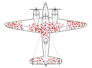
An important validity issue in applied econometrics is whether the sample used in the analysis may have a selection issue. Selection refers to the process by which the sample comes to be observed. Who or what entities were selected for observation, and was there a process that selected observations partly due to their levels of the outcome variable. This issue is sometimes called “sample selection” or “sample self-selection.” Self-selection is a general characteristic of social relationships and social processes. Figure 1 is a well-known illustration. The apocryphal story accompanying the illustration goes as follows. During WWII aircraft engineers wanted to better design bombers to improve their chances when flying through fields of anti-aircraft fire, or when attached by enemy fighter places. They recorded the bullet holes and other damage to aircraft returning to base. The figure illustrates the frequency of damage on different part of the returning planes. The engineers decided to reinforce those parts with lots of damage. But, just before the work started, a voice piped up, ”Wait a second, we’ve been looking at the sample that survived! The aircraft that crashed probably had damage precisely in those parts of the place (engines, cockpit, and rear fuselage). That is probably why they crashed and did not return. Those are the places that should be reinforced.”
The general point is that units of observation may be self-selected, and the self-selection may be based on the outcome that is being explained. This might arise because some person refuse to respond or participate in surveys; some people may drop out of the labor market; some countries might be defeated in war and no longer exist; some firms go bankrupt and stop operating; some young people drop out of school and are no longer tested; many homeless persons are uncounted in the national census; political polls miss people without telephones.
It can shown with some algebra that if the process determining inclusion in the sample depends on the outcome variable Y , after controlling for any influence of the explanatory variables on inclusion, then estimated coefficient may be biased. The bias will be larger the more the inclusion or exclusion is correlated with the outcome variable.
11.3.9 Externally valid estimation
External validity refers to the assessment of whether inferences about relationships estimated can be generalized from the population and setting studied to other populations and settings. The effect of changing social institutions towards more gender equal norms and attitudes on overall income per capita, estimated for a sample of African countries, may not be close to the effect of changed gender norms in Pacific Island nations. The effect of smaller class sizes in Tennessee, on student test scores, may be quite different from the effect of smaller class sizes in Brazil.
There are no statistical tests for external validity. One can use contextual knowledge and structured reasoning to arrive at a determination of the degree of likely external validity. More importantly, the community of social science needs to encourage and promote replications of important econometric studies, in other populations and settings, in order to determine external validity. Very often such replication exercises remain unpublished, and the community of social scientists continues to mention and draw lessons from a single study that may have little external validity.
11.4 Robust estimation
Social scientists increasingly recognize that they face a “garden of forking paths” when conducting their analysis. That is, any particular analysis often involves, literally, hundreds of small choices about cleaning, manipulating, and analyzing data. By the mathematics of permutations, this means there will be very many combinations of choices. Some of these combinations, by chance, will mean that an estimated coefficient will be statistically significant (or not significant). Some of the combinations, by chance, will generate an economically large (or small) coefficient.
The practice of “checking for robustness,” as it has come to be known, means presenting to the reader a variety or range of possible choices, and showing that the estimated coefficient on the variable of interest (the relationship of interest) maintains the same rough level of statistical significance and the same rough magnitude. That is, the many choices made in the data analysis appear not to have affected the result.
There are several ways to assure the community of social scientists of the robustness of results presented in a research paper.
First, the data and analysis code should, to be extent possible, be made publicly available so that other social scientists can replicate the original analysis and make different data wrangling choices (that are also reasonable) and see for themselves whether the coefficient of interest and its statistical significance changes by a substantial amount. Increasingly, this practice of making replication data available is required by academic journals that publish research articles. There are many online and publicly accessible repositories for data and code. Moreover, various organizations organize, periodically, replication exercises, where tens of hundreds of social scientists simultaneously replicate social science research, and examine robustness to their own reasonable data analysis choices.
Second, authors should leverage online accessibility and present online appendices with extensive checks for robustness. While a published, referees research article might have one table of regression results, an online appendix can easily (and cheaply) have ten tables of regression results, with many variations of included variables, specifications, alternative choices about measurement, corrections for sample selection, and other checks of robustness.
Third, to the extent possible, research articles could be paired, or could include two different data sources from two different contexts, to address questions about external validity, or “data venue shopping.” In data venue shopping, a researcher has a particular point of view that they wish to confirm (by finding a particular range of values or statistical significance for an estimated coefficient) and so they try different datasets until they find the one that, by chance, produces the result they hope to find.
Fourth, research can now be pre-registered before analysis is actually conducted. The pre-registration plan must be publicly available so that the community of social scientists can verify conformity of the final analysis with the plan. This works especially well for cases where original data will be collected. The analyst pre-specifies what regressions they will run and how variables will be measured and what data cleaning will be carried out. It works less well for standard, publicly available datasets, since the researcher can simply do data-mining in advance, obtain the results they wish, and then act as if they had done no analysis and pre-register the analysis and then, lo and behold, they find the results they had already found.
11.4.1 Examples of regressions that might be examined for validity
It can be a very useful exercise, at this point in one’s understanding of regression analysis, to examine the validity of regressions that one might encounter as a social scientist. What follows are three examples. In each example, we want to first think of the entity of observation. Validity issues might depend on the entity that is the unit of analysis.
11.4.2 Policing and crime
We imagine a measure of policing efficacy (number of sworn police officers) as the X variable and the crime rate as the Y variable. The entity of observation could be a at the neighborhood or precinct level, the city level, or county, or state, or country level. The different entities of observation will likely have different kinds of measurement error, influencing the judgment about the relevance of measurement error in the X variable in producing attenuation bias. We might also note that a measure of the police force might be a mismeasure of police efficacy. Other measures of efficacy include funding, training, or aggregate objective ratings of officers. We might think that reverse causality (simultaneous causality) is an important validity issue here: higher crime rates likely influence the size and efficacy of the local police force. Moreover, it is fairly easy to come up with a variety of omitted variables that satisfy the two-part test for producing OVB.
11.4.3 Car driving and CO2 emissions
In the era of climate change, social scientists and climate scientists are quite interested in measuring the relationship between car driving and the extent of carbon dioxide \(CO_2\) emissions. Automobile emissions are a major source of emissions, but they are generated by the choices of billions of people around the world about where to live, how to commute to work, and about how to enjoy leisure time. At the same time, governments are choosing how much to invest and maintain road and public transport infrastructure, and business are making similar decisions. Moreover, the mix of automobiles, and hence emissions per mile travelled, is constantly changing. It is an important relationship, but a hard one to estimate (or even to theorize exactly what one means by the relationship).
Suppose that an analysis has measured \(CO_2\) emissions and miles driven for a cross-section of observations. The entity of observation could be individual cars, or car brands, or households (where car trip of commuting decisions are made) , or county (where emissions are often measured), or state, or country. Practical issue of measuring car trips, car miles, and emissions have changed with advent of computerized sensors in vehicles that can wirelessly connect to networks, and with smartphones that track movements of people.
What are the validity issues with such a simple single variable regression? One can immediately think of simultaneous causality: perhaps areas where people know more about the consequences of their emissions are more likely to change their car trips! Indeed, one of the goals of climate change awareness is to have people calculate the emissions of their personal automobile trips (and other transport alternatives). Omitted variables are again likely to be a problem: people living in hilly areas, where cars have to engage a lot of power to go up hills, will have different patterns of trips and also different levels of emissions. Sample selection might be an important issue here, as people and places may choose to restrict trips by private automobile. Would a car-free city be included in the sample?
11.4.4 Gender of children and labor force participation
In countries all over the world, a major macroeconomic issue is the extent of labor force participation, and especially the participation of women, whose participation rates are almost everywhere lower than those of men, and whose participation rates fluctuate over the course of the business cycle.
There are many factors that explain variation across individual women or across societies, and over time, in participation rates. But consider variation at the individual level. A demographer, a sociologist, a feminist economist, or a labor economist might be interested in explanations at the gender norm level. One angle in exploring how norms matter for labor force participation might be to examine the relationship between labor force participation and the gender composition of children of a parent, especially of a female parent. The gender mix of children is random, to some degree. We write “to some degree” because some parents may engage in pre-term sex selective abortion. Moreover, some parents may change their fertility behavior depending on the gender of previously born children. In societies with strong preference for sons, parents who have two girls might try to have another baby, even though if they had had two sons, or a son and daughter, they might be satisfied with just two children.
We see immediately then that estimating a relationship at the individual level, with sex composition of children as the explanatory variable and a binary outcome variable of whether the mother is working, will have a sample selection problem. Many women will have no children. They cannot be in the sample, since there is no measure of the gender of their children. One can think of measurement issues, of simultaneous causality (some women may be working more than they would to pay for fertility treatments), and plenty of omitted variables.
11.5 Concluding thoughts
Discussions about credibility should try to reflect and incorporate a shared understanding of the purposes of estimating a particular causal relationship. Who might be affected by an unbelievable or incredible estimation? How much might they be affected? The more serious the answer to those questions, the more scrutiny and consideration should be brought to discussions about validity and robustness.
Currently, statistical computing software (such as R or Stata) can estimate coefficients and associated standard errors for any outcome variable, set of explanatory variables, and specification. It is not far-fetched to imagine a near future where any regression estimated using statistical computing software comes with an AI-generated text that offers interpretation and contextualization about the believability of regression results. Such AI software, we can imagine, might “read” this chapter and anticipate the believability issues raised and apply them to any particular regression and generate coherent text. We can imagine a sort of conversation with such an AI, where we ask it questions about the regression, and the AI generates answers. Perhaps the AI might adopt the voice of Cormac McCarthy? Review terms and concepts: • internal validity • external validity • misspecification • credibility • identification strategies • imperfect multicollinearity • measurement error • simultaneous causality • sample selection bias • robustness