8 Understanding omitted variable bias
Abstract
This chapter covers the concept of omitted variable bias (OVB), or confounding, in regression analysis. The emphasis is on developing the intuition of how and why an omitted variable biases the estimated coefficient on a variable of interest. The chapter provides numerous examples of regressions that likely suffer from OVB, and works through the logical reasoning needed to predict the direction of bias.
Keywords: Omitted variable bias, confounder
8.1 Omitted variable bias
Previous chapters have examined the single variable and multiple variable regression model. A variable \(X_1\) is hypothesized to affect an outcome \(Y\). Other control variables \(X_2,X_3,X_4\) are also included in the regression as explanatory variables, because they are also hypothesized to affect the outcome \(Y\). The explanatory variable \(X_1\) is assumed to be independent of, or uncorrelated with, any other factors influencing the outcome, or systematic measurement error of the outcome, once the other control variables are taken into account. This assumption is expressed mathematically as \(E(ϵ_i|X_1,X_2,X_3,X_4) = 0\); the expected error term is assumed to be equal to zero, conditional on the level of the explanatory variables.
The assumption would be violated if one or more other factors influencing the outcome that are not included (“omitted”) in the regression were correlated with the level of the explanatory variable of interest \(X_1\). These possible omitted variables are often called “confounders.”
Omitted variable bias (OVB) arises, and becomes a concern, when an analyst examining or thinking about a proposed regression model considers a two-part test: first, is there a likely omitted explanatory variable that is correlated with the included \(X_1\) variable of interest; and, second, does this omitted variable independently have a causal effect on the outcome \(Y\). An estimated regression coefficient is said to “suffer” from OVB when one can reasonably identify such an omitted variable. The bias arises only when both conditions are met.
In this chapter, we focus on OVB in the single variable regression case. We develop the intuition about how to deduce the likely direction of bias: How will specific instances of OVB change the estimated coefficient, in terms of the sign and magnitude? The intuition of how omitted variables might bias estimated coefficients in the multiple regression case is not as easily discerned. With some simplifying assumptions about the included variables, however, it is possible to have more intuition (Clarke, 2019). But in general the direction of the bias for the coefficient of the variable of interest will depend on the full set of correlations among the included explanatory variables and the omitted variable, and so cannot be readily discerned. For that reason, we focus on the single variable case.
8.2 OVB in the Mincer education-earnings relationship
The simple Mincer equation for estimating the earnings and education relationship has log earnings as the outcome variable and education as the explanatory variable of interest: \(logearn_i = β_0 + β_1educ_i + ϵ_i\). Recall that the error term \(ϵ_i\) is intended to capture the influence of all the other factors that affect a person’s earnings, beside their education. So far in this course we have assumed that this error term is independent of the regressor, \(educ: E(ϵ_i|education) = 0\). The assumption of \(E(ϵi|education) = 0\) could be violated if an attribute of individuals, such as their general aptitude or ability to master complex knowledge activities, were omitted from the regression. Such ability might vary across individuals. It might be measurable through various general-purpose intelligence or aptitude tests. But it might not be available in the dataset at hand. Because ability is unobserved and cannot be included in the regression, its absence will confound the estimate of the effect of education on earnings.
Will the omission of this variable be a problem? Yes! The estimate of the coefficient on education would likely be biased because part of the estimated coefficient is plausibly attributable to the ability “other factor” which is correlated with education and which likely influences the outcome, earnings. That is, it will look like high education causes a person to have high earnings; but the correlation is partly an illusion, because high ability is likely to cause both high education and high earnings. That is, even if they did not have high educational attainment, people with high ability would likely have high earnings. This is what we mean when we say that the estimate of the coefficient on education will likely be biased as an estimate of the causal influence of education on earnings.
Figure 1 may be helpful in understanding the direction of the bias. Figures like this are often called Directed Acyclic Graphs (DAG). A DAG has nodes and lines with arrows connecting the nodes. The lines and arrows indicate the pathways of causality and correlation, or sometimes both. For more on DAGs, see the discussion in Imbens (2020) and Huntington-Klein (2022), and the website https://dagitty.net/learn/graphs/roles.html. In the case of Figure 8.1, the nodes are earnings, education, and ability. Education and ability causes earnings, but ability also causes education, and education is thus correlated with ability.
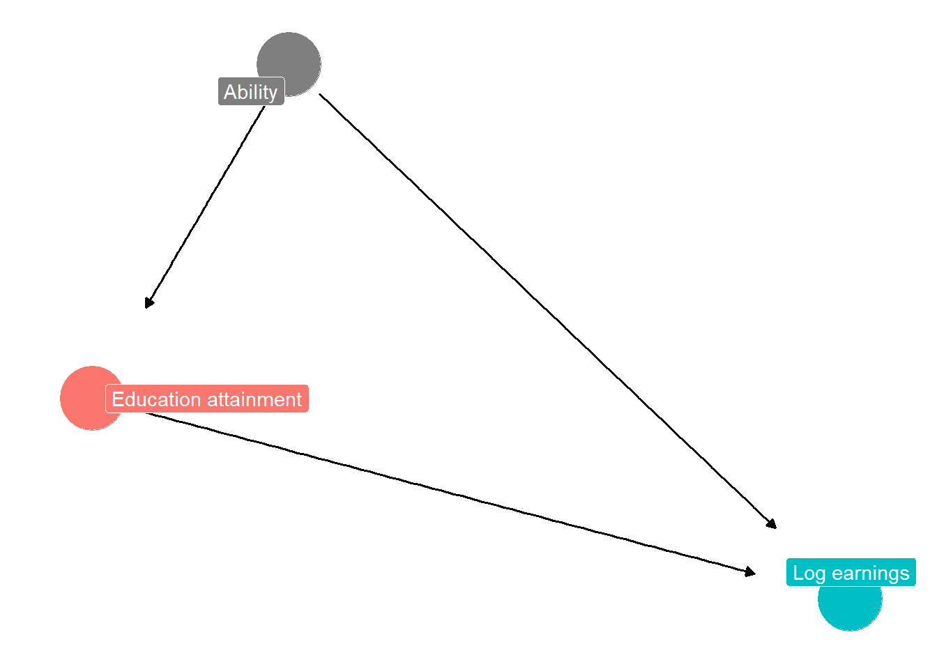
Figure 8.1: DAG diagram illustrating how an omitted variable (a confounder) can bias estimate of effect of education on earnings
Ordinarily, we might expect a positive relationship between education and log earnings. The coefficient representing the true relationship might be, for example, .10. Each one unit increase in education increases earnings by 10%. In estimating the single variable regression, however, ability may plausibly be an omitted variable. Ability might be positively correlated with education, and might also lead to higher earnings. Because the variable is omitted from the regression, the estimated coefficient on education will be a larger positive number than it should be; it might be .15. It looks like individuals with high education have quite high earnings. But this is only partly because high education increases earnings; it is also partly because individuals with high education also have high ability, and ability increases earnings. The estimated coefficient would be smaller (in absolute value) if ability were controlled for by including a measure of ability in the regression. Then the coefficient on education would be estimated as .10.
We have focused on one possible omitted variable, ability, but of course there are many other possible omitted variables. Table 8.1 may be helpful in thinking through the different possibilities. We imagine there are four different possibilities of the omitted variable in a regression with earnings as the outcome and education attainment as the explanatory variable. In the first case, ability is the omitted variable, the confounder. In the second case, some people are more “dreamily intellectual” than others. In the third case, some people are more likely to embody what is colloquially called “hustle culture.” In the fourth case, some people are more inclined to smoke a lot of weed during and after their youth (when aged 15-30, say).
| What is omitted variable Z (the confounder)? | Sign of correlation between education attainment and Z | Sign of effect of Z on earnings | \(\beta\) true | \(\beta\) could be … if Z omitted |
|---|---|---|---|---|
| ability | \(+\) | \(+\) | .10 | .15 |
| dreamily intellectual | \(+\) | \(-\) | .10 | .05 |
| hustle culture | \(-\) | \(+\) | .10 | .05 |
| smokes lots of weed | \(-\) | \(-\) | .10 | .15 |
In the first case, the omitted variable or confounder, as noted, results in a biased estimate of the coefficient. One might estimate an effect of education on log earnings of .15, when the true parameter was .10.
In the second case, we might see a potential underestimate of the true relationship between education and earnings. The estimated coefficient could be .05. It might seem that education does not affect earnings that much. The reason is that people who have high education attainment tend to be more “dreamily intellectual” and decide to write obscure, highly literary novels, or poetry, or modernist classical music, or work saving the beluga whale, and so they do not earn as much as their peers, even those with less education who find satisfaction in more lucrative occupations.
In the third case, we again underestimate the true relationship between education and earnings, but this time for a different reason. Now people with low education attainment are more likely to be those who have an aptitude as entrepreneurs; they are impatient with theoretical knowledge and instead immediately pursue practical knowledge of “how to make a dollar” that is not taught in school. They seek out mentors and network with other hustlers. Low education adults, then, may disproportionately include such types of persons, and so they earn more than they might be expected to, given their low levels of education. So, while education is valuable (the true coefficient is .10) its return is estimated to be lower, perhaps only .05. Finally, the fourth case, like the first, is consistent with an over-estimate of the return to education. Here, low education people are also people who smoke a lot of marijuana. In the traditional stereotype of such individuals they are slackers and unambitious, not too concerned about making money, and appear to enjoy “hanging out” more. The estimated return to education appears to be high. The marijuana smokers drop out of school early, not to earn money, but to hang out and get high. Low education attainers appear to earn even less than they might, because they are disproportionately low-achieving pot smokers.
It seems quite plausible that all of these omitted variables, each introducing its own OVB, could be at work in our simple estimate of the return to education. The net effect, and the net direction of the bias, will depend on a complex set of factors, such as the strength of the correlations in each case, and how many people in our sample are “dreamy intellectual” types versus hustling entrepreneurs.
8.3 Two other examples of OVB
Consider two other examples of single variable regressions where an omitted variable might be associated with bias of the estimated coefficient on the variable of interest.
The first example concerns an old big question in social science and history: What was the impact of European expansion, settlement, and colonialism in the almost 500 year period 1500-1960 of European imperialism on the incomes and well-being of people in the affected regions. One smaller version of the question is this: Did regions that saw more European settlement end up in the year 2000 with higher or lower incomes per capita, relative to regions that saw less European settlement?
Let us remark that both the big question and the small question are a bit incoherent. If European settlement led to the complete decimation of native peoples (as, for example, in some Caribbean islands), what is the sense of measuring income per capita in the present as an outcome?
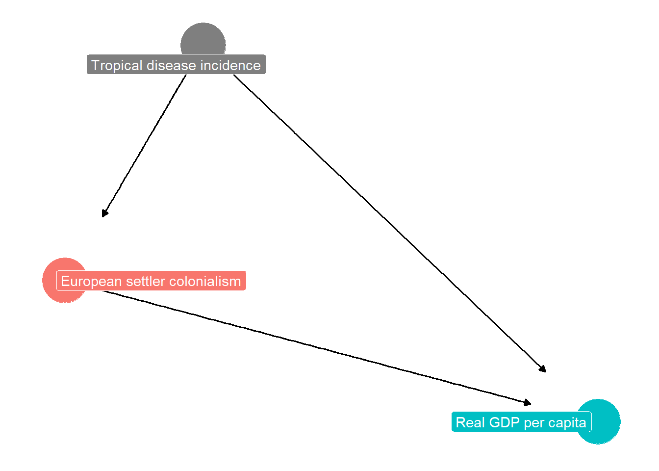
Figure 8.2: DAG diagram illustrating how an omitted variable (a confounder) can bias estimate of effect of European settler colonialism on the level of real GDP per capita
Nevertheless, regression analysis proceeds! And it has an omitted variable problem. The confounder problem with the regression is illustrated in Figure 8.2. We can imagine estimating a relationship where the outcome variable is “current GDP per capita” and the explanatory variable is “extent of European settlement in region during era of imperialism.” Suppose we estimate a positive coefficient. Did European settlement indeed lead to higher GDP?
As the DAG suggests, we might think an omitted variable or confounder is “tropical disease incidence” with higher numbers of the index indicating a more tropical climate with more infectious diseases. This variable negatively determines GDP, and also likely negatively affected European settlement. The variable meets the two-part test for OVB. So we see the estimated coefficient is biased upwards, and the “actual” or unbiased effect of European settlement is smaller, or perhaps negative, relative to what we have estimated.
We can see that a tricky situation arises when the bias is large enough that the sign is reversed! European settlement could actually have had a true negative effect on subsequent GDP, but the biased coefficient is positive because Europeans strongly avoided tropical areas with high disease incidence which might generally have lower GDP than temperate areas. In other words, European settlement reduced GDP growth (from what it could have been) in temperate areas, just not enough to make subsequent GDP actually lower than tropical GDP levels.
It takes awhile for most people to get the hang of OVB analysis, because it consists of taking into account three “signs.” First is the sign, positive or negative, of the true relationship between the included \(X\) and the outcome \(Y\) ; second is the sign of the correlation between \(X\) and \(Z\); and third is the sign of the true relationship between \(Z\) and the outcome \(Y\) . In understanding the intuition, it helps to start by assuming that the relationships are such that the sign of the effect of interest is never flipped; that is, magnitudes and signs are not such that OVB could actually cause the sign on the included \(X\) to flip. OVB big enough to flip the sign of the estimate is certainly possible and indeed happens frequently in econometrics. But for the intuition, it is better to start with simpler cases.
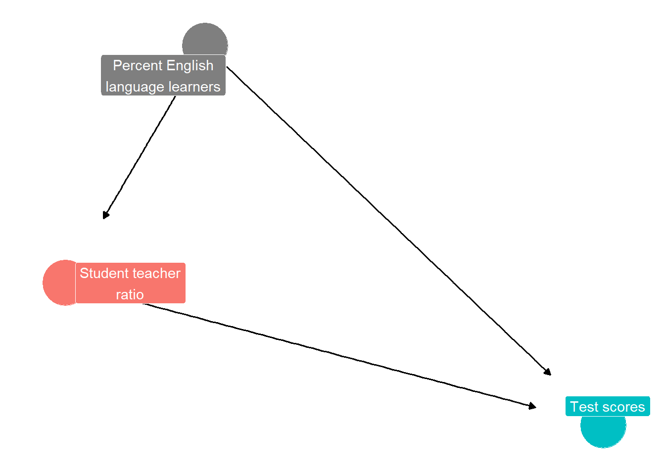
Figure 8.3: DAG diagram illustrating how an omitted variable (a confounder) can bias estimate of effect of student teacher ratio on school district test scoress
Consider another example, illustrated by the DAG in Figure 8.3. We imagine we have data on the student-teacher ratios for middle schools in all school districts in a state, or in a country. The ratios might vary from a low of 12 students per teacher to a high of 35 students per teacher. We also might have data on average scores in reading and math for middle school students, from a standardized text.
Ordinarily, we might expect a negative relationship between higher student teacher ratio in a school district and the average test score for the district. Too many students, and teacher and students are distracted and so students do not learn well. The coefficient representing the true relationship might be, for example, -2.28. Each one unit increase in the student teacher ratio reduces the district test score by 2.28.
In estimating the single variable regression, however, the percent English language learners in each district may plausibly be an omitted variable, or confounder. English language learners are students whose parents do not speak English at home. These students spend much of primary school learning English, and so they may be a little behind when they reach middle school. Some English language learners may have moved from abroad and are starting school in the United States in middle school, knowing very little English.
The percent English language learners might be positively correlated with the likelihood of the district having a high student teacher ratio, and might also be associated with lower test scores. English language learners are less likely to perform well on a test that is all in English. Because the variable is omitted from the regression, however, the estimated coefficient on the student teacher ratio may be a larger negative number than it should be; it might be -4.28. It looks like counties with high student teacher ratios have very low test scores. But this is only partly because student teacher ratios reduce test scores; it is partly because districts with high student teacher ratios have high percent English language learners. The estimated coefficient - 4.28 would be smaller in absolute value (less negative) if the percent English language learners were controlled for by including it in the regression. Then the coefficient would be estimated as -2.28.
8.4 A general framing of OVB
In general, to determine the direction of potential omitted variable bias (will the biased coefficient be larger or smaller in absolute value than the true coefficient), one asks two questions (the two-part test): (1) how is the omitted variable correlated with the included variables; and (2) how might the omitted variable affect the outcome, on its own. These two considerations determine the correlation between the error term and the included X variable, given by \(ρ_{Xϵ}\). Indeed, it is straightforward to show that if \(E(ϵi|Xi)\neq 0\), then, \[ \hat{\beta_1} \xrightarrow{p} \beta_1 + ρ_{Xϵ} \frac{\sigma_\epsilon}{\sigma_X}\] (8.1)
where \(σ_ϵ\) is the standard deviation of the error term, \(σ_X\) is the standard deviation of the regressor \(X\), and \(ρ_{Xϵ}\) is the correlation between \(X\) and \(ϵ\). The second term (after the +) represents the bias, because it is the difference between the “true” coefficient \(β_1\) and the biased estimate \(\hat{\beta_1}\). Box 8.1 contains a proof of this result.
Table 2, a generalization of our earlier table, may be helpful in thinking through the different possibilities, dealing with cases where the true coefficient could be either positive or negative.
| Suppose true X Y coefficient were… | Suppose correlation between X and Z were… |
Suppose Z affects Y…
the equation) might be..
|
The unbiased estimated (obtained by including Z in the
regression and reestimating) might have been.
|
|||
|---|---|---|---|---|---|---|
| 1 | positive | positive | positively | \(+\) | 6.4 | 4.4 |
| 2 | negatively | \(-\) | 6.4 | 8.4 | ||
| 3 | negative | positively | \(-\) | 6.4 | 8.4 | |
| 4 | negatively | \(+\) | 6.4 | 4.4 | ||
| 5 | negative | positive | positively | \(+\) | 6.4 | -8.4 |
| 6 | negatively | \(-\) | 6.4 | -4.4 | ||
| 7 | negative | positively | \(-\) | 6.4 | -4.4 | |
| 8 | negatively | \(+\) | 6.4 | -8.4 |
Consider for example the case of a true negative relationship (such as that between student-teacher ratio and test scores). Now imagine an omitted variable that is exposure to air pollution in the school district. Air pollution negatively directly influences test scores, on average. Moreover, teachers may be reluctant to live and teach in school districts where they themselves are exposed to air pollution, so class sizes might, on average, be larger. More air pollution thus means larger class sizes, or larger student-teacher ratios.
We are thus in case 6 towards the bottom of the table, with a negative true effect of \(X\) on \(Y\), a positive correlation between \(X\) and \(Z\), and a negative relationship between \(Z\) and \(Y\). The correlation between \(X\) and \(ϵ\) (namely, \(ρ_{Xϵ}\)) is negative: when \(X\) is bigger, \(Z\) tends to be bigger, and when \(Z\) is bigger, the omitted error term \(ϵ\) tends to be smaller. A simple regression of test scores (\(Y\)) on student-teacher ratio (\(X\)) might yield an estimated coefficient of -6.4. Thus it appears that larger class size negatively affects test scores by a lot. But if air pollution could be measured and included in the regression, the true coefficient on class size would be -4.4, not as large in absolute value. The single variable regression suffers from OVB. It appears that class size negatively impacts test scores more than it actually does, because part of the negative effect of class size is really the negative effect of air pollution, which is higher in places with larger class size.
Notice again that we use numeric examples of how the coefficient might change. This is because in English for a negative coefficient it is awkward to say things like “it will go up” because an increase in absolute value means the coefficient is smaller (a larger negative number). To avoid that ambiguity, it is better to use a numeric example when explaining the direction of bias.
Box 8.1: Derivation of the formula for bias of OLS coefficient in single variable regression case
We start by taking the expectation of the estimator for the slope coefficient, conditional on the X variables:
\[\begin{equation} E(\widehat{\beta_1}|X) = E( \frac{\sum_{i = 1}^N \left( x_i - \overline{x} \right) \left( y_i - \overline{y} \right)}{\sum_{i = 1}^N \left( x_i - \overline{x} \right)^2} | X) \end{equation}\] We can substitute in the true population regression model for the \(y_i\) and \(\overline{y}\): \[\begin{equation} E(\widehat{\beta_1}|X) = E( \frac{\sum_{i = 1}^N \left( x_i - \overline{x} \right) \left( \beta_0+\beta_1x_i+\epsilon_i - \beta_0-\beta_1 \overline{x} - \overline{\epsilon} \right)}{\sum_{i = 1}^N \left( x_i - \overline{x} \right)^2} | X) \end{equation}\] We can cancel the \(\beta_0\), \[\begin{equation} E(\widehat{\beta_1}|X) = E( \frac{\sum_{i = 1}^N \left( x_i - \overline{x} \right) \left(\beta_1x_i+\epsilon_i -\beta_1 \overline{x} - \overline{\epsilon} \right)}{\sum_{i = 1}^N \left( x_i - \overline{x} \right)^2} | X) \end{equation}\] Rearranging, \[\begin{equation} E(\widehat{\beta_1}|X) = E( \frac{\sum_{i = 1}^N \left( x_i - \overline{x} \right) \left(\beta_1 (x_i-\overline{x})+\epsilon_i- \overline{\epsilon} \right)}{\sum_{i = 1}^N \left( x_i - \overline{x} \right)^2} | X) \end{equation}\] More rearranging, \[\begin{equation} E(\widehat{\beta_1}|X) = E( \frac{\sum_{i = 1}^N \beta_1 \left( x_i - \overline{x} \right)^2} {\sum_{i = 1}^N \left( x_i - \overline{x} \right)^2} + \frac{\sum_{i = 1}^N \left( x_i - \overline{x} \right)\epsilon_i}{\sum_{i = 1}^N \left( x_i - \overline{x} - \right)^2} - \frac{\sum_{i = 1}^N \left( x_i - \overline{x} \right) \overline\epsilon}{\sum_{i = 1}^N \left( x_i - \overline{x} - \right)^2}| X) \end{equation}\] Or, since $ (_{i = 1}^N ( x_i - ))=0$ by the definition of \(\overline{x}\), \[\begin{equation} E(\widehat{\beta_1}|X) = E(\beta_1 \frac{\sum_{i = 1}^N \left( x_i - \overline{x} \right)^2} {\sum_{i = 1}^N \left( x_i - \overline{x} \right)^2} + \frac{\sum_{i = 1}^N \left( x_i - \overline{x} \right)\epsilon_i}{\sum_{i = 1}^N \left( x_i - \overline{x} \right)^2} | X) \end{equation}\] Or, \[\begin{equation} E(\widehat{\beta_1}|X) = E(\beta_1 + \frac{\sum_{i = 1}^N \left( x_i - \overline{x} \right)\epsilon_i}{\sum_{i = 1}^N \left( x_i - \overline{x} \right)^2} | X) \end{equation}\] Or, \[\begin{equation} E(\widehat{\beta_1}|X) = \beta_1 + E(\frac{\sum_{i = 1}^N \left( x_i - \overline{x} \right)\epsilon_i}{\sum_{i = 1}^N \left( x_i - \overline{x} \right)^2} | X) \end{equation}\] Now if the error term were uncorrelated with the \(x_i\) the second term would be zero. But without that assumption, it cannot be assumed to be zero. With some algebra and using the Law of iterated expectations (that the expected value of a random variable is equal to the sum of the expected values of that random variable conditioned on a second random variable), we can arrive at: \[\begin{equation} \widehat\beta_1 \xrightarrow[]{p} \beta_1 + \rho_{X\epsilon} \frac{\sigma_\epsilon}{\sigma_X}. \tag{8.1} \end{equation}\]
8.5 Two more examples of OVB
8.5.1 The relationship between gender of college athletic director and baseball team performance
Suppose you have a sample of 820 public and private universities in the United States that report their data to the fictitious Gender Equality in Universities Project. Suppose that the following variables are included in this imaginary dataset: \(Perf\) = Performance of men’s university baseball team over season (i.e., proportion wins); \(Highincome\) = Proportion high income students attending university; and \(Femathdir\) = Dummy variable if overall athletic director of school is female. You are interested in whether having a female athletic director in general has an effect on the performance of the men’s baseball team. You estimate a regression and obtain the following coefficients (assume they are statistically significant): \(Perf = .50 − .06 ∗ Highincome + .13 ∗ Femathdir\).
Could omitted variable bias affect the estimated regression coefficient on \(Femathdir\)?
To answer this question, one needs to ask whether there is a variable that is likely correlated with whether a university has a female athletic director and that also is likely to cause (in a logically coherent way) the outcome, the performance of the men’s baseball team. That is, you must propose an omitted variable \(Z\) and say how it would bias the coefficient. If the bias on \(Femathdir\) were corrected by including the omitted variable \(Z\) in the regression, according to your understanding of the omitted variable and assumptions about correlations, would the coefficient on \(Femathdir\) go from, say, .13 to .33, or rather to .03?
There is no single right answer. Rather, there are many plausible right answers, or rather, variables that might meet the two-part test for OVB. For example, perhaps private religious universities attract lots of talented men baseball players, for historical reasons. They also may compensate for over-representation of men in top leadership positions at the university by selecting a female athletic director (leadership at most religious universities is male-heavy, sometimes explicitly so in their bylaws because they require that the president, provost, and chancellor positions be clergy, who are more likely to be male). We now have a logically coherent, and perhaps plausible, account for a correlation between whether a university has a female athletic director and whether a university attracts a good pool of male talent for the men’s baseball team, which in turn explains the successful season of the team. As a causal explanation of the baseball team’s success, the coefficient on female athletic director suffers from omitted variable bias. If the religious affiliation of universities were an included, instead of omitted, variable, we might expect the coefficient on \(Femathdir\) to go down to .03, for example.
Incidentally, since college athletics is such a big business for universities, this broad area of gender representation in athletics is a growing area of research Darvin and Demara (2021); Lancaster (2018); Mitchell (2020); Kimura (2018).
There are also wrong answers, that the consensus of people with good understanding of universities and econometrics would agree would not be sources of bias. For example, suppose someone said that they thought that the proportion of students at universities who were Economics majors was an omitted variable, biasing the coefficient on female athletic director. Most persons would agree that it would be a struggle to come up with a coherent story that was plausible in the context of U.S. higher education in the 2000s for why the proportion of Economics majors would be correlated with whether the university had a female athletic director and also explained the performance of the men’s baseball team.
8.6 A tale of two (or three) regressions
We have seen that OVB in an estimate of the slope coefficient arises when we have omitted an explanatory variable \(Z\) that independently partly determines the outcome variable \(Y\) and is correlated with the included regressor \(X\). This suggests that adding the omitted variable Z as a regressor—if we had it in our data—would resolve or mitigate the OVB. Let’s compare these two regressions: one omitting \(Z\), and one including it.
The simple regression of \(Y\) on \(X\), omitting \(Z\), can be called the “short” regression—we use the superscript \(S\) to stand for short here: \[Y_i = \beta_0^S + \beta_1^S X_i + \epsilon_i^S\]
The “long” regression is the multiple regression that adds the omitted regressor Z to the short regression, with the superscript \(ℓ\) standing for long : \[Y_i = β^ℓ_0 + β^ℓ_1 X_i + β^ℓ_2 Z_i + ϵ^ℓ_i\] As you might expect, the estimates of the slopes \(β^S_1\) and \(β^ℓ_1\) from these regressions will be different when there is OVB in the short regression, and their relationship can be derived from the same algebra that underlies the formula for OVB given in equation 8.1 that is developed in Box 8.1. Specifically, it turns out that \[\beta_1^S = β^ℓ_1 + β^ℓ_2\pi_{ZX}\] In this expression for the short regression slope, the first term \(β^ℓ_1\) represents the direct (causal) effect of \(X\) on \(Y\), and the second term \(β^ℓ_2π_{ZX}\) represents the OVB, driving a “wedge” between the short and long estimates of \(β_1\). The OVB term in turn has two components. \(β^ℓ_2\) is the coefficient on \(Z\) in our long (multiple) regression. But what is \(π_{ZX}\)? \(π_{ZX}\) is the slope of a third “auxiliary” regression where we regress \(Z\) on \(X\). Thus, it captures the relationship between the omitted regressor \(Z\) and the included regressor \(X\). The OVB is thus the product of two terms that together determine the impact of omitting the omitted variable: the relationship between \(Z\) and \(Y\), and the relationship between \(X\) and \(Z\). Only if both are non-zero will the short regression suffer from OVB.
Using the Kenya earnings data, we can run a real example of the long and short regressions to check if it works. In Table 3, the first—short—regression regresses log of earnings on a dummy variable for rural. The slope gives us \(\hat{\beta}^S_1 = −0.668\). You can see that the result implies a very large average earnings penalty for rural dwellers, with a coefficient of -0.668 “log points” (roughly 67% lower earnings). One might suspect that a contributing factor to that difference is that rural Kenyans may have less completed education, as is true of rural folks in much of the world. The second regression adds years of education as a regressor, giving us the long regression estimates \(\hat{\beta}^l_1 = −0.451\) and \(\hat{beta}_2^l = 0.117\). You can see that the rural earnings disadvantage remains large and negative, but is now smaller in magnitude.
To check the OVB calculation, we need to run the third—auxiliary— regression of the omitted variable \(educ\_yrs\) on the included regressor \(rural\), which is displayed in the third regression column. The slope is our estimate of \(\hat{\pi}_{ZX} = −1.848\). Now we have all the ingredients:
\(\beta_1^S = \beta_1^l + \beta_2^l \pi_{ZX} = -0.451 + 0.117 \cdot -1.848 = -0.667\), which is indeed the short regression coefficient, within rounding error.
8.7 Yet another way to think about OVB
A technique that may be helpful is to draw, on a graph, the hypothesized true linear relationship between \(X\) and \(Y\) in the single variable regression case. Normally the errors would be distributed evenly around this hypothesized line. The actual observations in a dataset would thus look evenly spread around the true relationship. The data satisfied the condition that for any given value of \(X\) the expected value of the errors is zero, \(E(ϵ|X) = 0\).
If there were OVB, however, then the errors in the single variable case would not satisfy the condition \(E(ϵ|X) = 0\). Then one imagines two possibilities: the errors are positively correlated with \(X\) so that high values of \(X\) are associated with relatively high values of \(Y\) , due to the omitted variable; or the errors are negatively correlated with \(X\) so that high values of \(X\) are associated with relatively low values of \(Y\) .
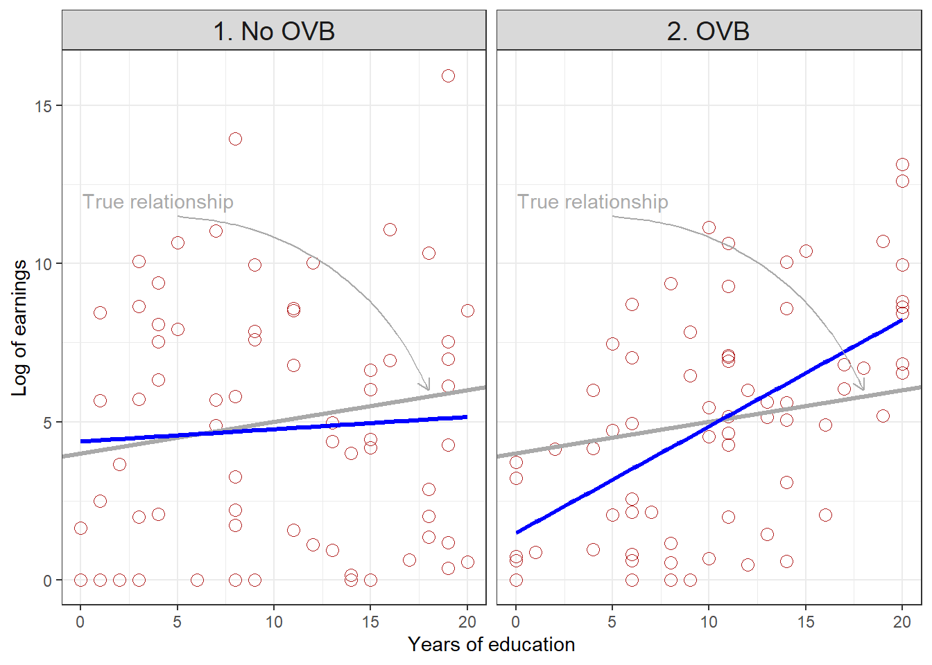
Figure 8.4: Scatterplots, true regression lines, and estimated regression lines under alternative assumptions about correlation between education and ability
Figure 4 illustrates the first possibility, in the context of our education and earnings example. The outcome is the log of earnings, and the explanatory variable of interest is years of education. The data have been simulated. In the left panel (1), earnings are determined by education and ability, but education and ability are not correlated, and thus \(E(ϵ|X) = 0\). The estimated regression line (blue) lies close to the true relationship between education and earnings (the gray line). In the right panel (2), earnings are determined by education, but education itself is partly determined by ability, and ability also directly affects earnings. Now, people with low ability have low levels of education. Notice that in the simulated data, all observations of people with 5 years of education or less have earnings “below” those predicted by the true regression relationship, because they have low ability that reduces their earnings. On the other hand, almost all people with education above 15 have earnings higher than those predicted by the true regression line, because they have high ability which boosts their earnings.
8.8 Subtle issues
It is worth mentioning two situations that are not called OVB. The first is when variables that are similar to the included variable of interest, in terms of what underlying conceptual variable they are measuring, are omitted. For example, consider an analyst who has data from a large sample of cities, and for each city the data has a variable for the overall non-violent crime rate in the city, and a variable for the number of shoplifting arrests, and a number for the reliance on and use of private security guards. These three variables are correlated, and connected causally by a complex simultaneous set of decisions by retail businesses, low-level criminal gangs, youth disaffection, political leadership, prosecutorial discretion, local journalism, etc. Very often, however, an applied economist is using one as a proxy variable for the other. The use of private security guards, or shoplifting arrests, may be taken as a proxy for the perhaps unmeasured overall non-violent crime rate. In any given application, two of the three variables would not be included in the regression, and yet this is not referred to as omitted variable bias. The situation, or variables, are sometimes called “proxy confounders.”
A similar, and often related situation, is when a researcher has access to “mediator” variables. Mediators are measures of outcomes that lie between the initial cause (the explanatory variable) and the final outcome (the Y variable). For example, consider again an analyst who has data from a large sample of cities, and now for each city the data has a variable for the nonviolent crime rate in the city, and a variable for the rate of arrests in the city, and a variable for the rate of successful prosecutions in the city. These variables are correlated, and connected causally by a complex simultaneous political economy of citizen engagement, political leadership, police union activism, local journalism, etc. Very often, however, an applied economist is using the successful prosecution rate as the outcome. The non-violent crime rate might be the explanatory variable of interest. The arrest rate is a mediating variable, leading to prosecutions. It should not be included as an explanatory variable in a simple regression. Much more complex regression models are needed when considering situations where mediating variables are important in explaining a social situation of interest.
As usual, we let the generative AI ChatGPT, simulating the voice of author Cormac McCarthy, clarify the distinctions (or not!).
In the sparse landscape of causal inference, where shadows stretch long and intentions are obscured, proxy confounders and mediator variables exist as specters, distinct yet entwined with the essence of true confounders. The true confounder, that wretched thing, stands as an uninvited guest at the table of observation, a variable that twists the path of cause and effect, entwining outcomes in its grasp. It hides in plain sight, a phantom driving the narratives we weave, distorting the light of truth. Proxy confounders, however, are like echoes in a canyon, distant and distorted. They stand in for the true confounders, offering a semblance of understanding while obscuring the deeper truths. They might lead one to think they’ve grasped the heart of a matter when, in truth, they are merely shadowboxing with phantoms. They reflect the complexities of the world, but they do so through a glass darkly, never quite capturing the essence of what lies beyond. Mediator variables, then, act as the conduit in this tangled web, the bridges that connect cause to effect. They are the channels through which the influence flows, the streams that carry the weight of causality. Yet, they too stand apart from the true confounders, for they do not obfuscate but rather clarify, revealing the pathways of influence while still being susceptible to the storms of external forces. In this unforgiving landscape of analysis, it is essential to recognize these distinctions, to sift through the sands of data and discern the true nature of these entities. The path to understanding is fraught with peril, where the lines between cause and consequence blur, and the true confounders lurk, waiting to lead the unwary astray.
Review terms and concepts: • confounder • omitted variable bias (OVB) • two-part test