4 Data Processing

4.1 Gene body coverage

The union transcript is used to extract only exon pileup. To keep only exon location, we first build coverage pileup from raw pileup (part_intron) to pileupData (only_exon). Let’s compare the dimension of pileup for the first and the last genes using get_pileupExon function: LINC01772 and MIR133A1HG have 3,245 and 5,825 positions, respectively.

genelist[c(1, length(genelist))]

## [1] "LINC01772"  "MIR133A1HG"

pileupPath <- paste0("./data/pileup/", genelist,"_pileup_part_intron.RData")
LI = get_pileupExon(g=1, pileupPath)
MI = get_pileupExon(g=length(genelist), pileupPath)
dim(LI); dim(MI)

## [1] 3245  171

## [1] 5825  171

Before coverage normalization, we identified and filtered low-expression genes in the filter_lowExpGenes function to reduce sampling noise. Only 961 out of 1,000 genes were used for gene body coverage by considering genes with smaller percentages of TPM < 5 than 50%. Genes were divided into two groups to compare coverage patterns in short and long genes. 0~5 kb and 5+ kb cover 96 and 865 genes, respectively.

# Filtered genes
genelist2 <- filter_lowExpGenes(genelist, TPM, thru=5, pct=50)
pileupPath2 <- paste0("./data/pileup/", genelist2,"_pileup_part_intron.RData")
length(pileupPath2)

## [1] 961

geneInfo2 <- geneInfo[match(genelist2, geneInfo$geneSymbol), ] %>%
  mutate(merged_kb=merged/1000,
         Len=factor(case_when(
           merged_kb>=0 & merged_kb<5 ~ "0~5 kb",
           merged_kb>=5 ~ "5+ kb",
           is.na(merged_kb) ~ NA)),
         LenSorted=forcats::fct_relevel(Len, "0~5 kb", "5+ kb")
  )

table(geneInfo2$LenSorted)

## 
## 0~5 kb  5+ kb 
##     96    865

genelist2Len0 <- geneInfo2[geneInfo2$LenSorted=="0~5 kb", c("geneSymbol")]
pileupPath2Len0 <- paste0("./data/pileup/", genelist2Len0,"_pileup_part_intron.RData")

genelist2Len5 <- geneInfo2[geneInfo2$LenSorted=="5+ kb", c("geneSymbol")]
pileupPath2Len5 <- paste0("./data/pileup/", genelist2Len5,"_pileup_part_intron.RData")

In the plot_GBC function, evenly spaced regions are defined as gene body percentile where the number of regions is 100. For details of the normalized coverage at the region, see Gene Length Normalization in the R functions.

GBC0 = plot_GBC(pileupPath2Len0, geneNames=genelist2Len0, rnum=100, method=1, scale=TRUE, stat=2, plot=TRUE, sampleInfo)
GBC5 = plot_GBC(pileupPath2Len5, geneNames=genelist2Len5, rnum=100, method=1, scale=TRUE, stat=2, plot=TRUE, sampleInfo)

p0 <- GBC0$plot +
  coord_cartesian(ylim=c(0, 0.017)) +
  ggtitle("0~5 kb")
p5 <- GBC5$plot +
  coord_cartesian(ylim=c(0, 0.017)) +
  ggtitle("5+ kb")

ggpubr::ggarrange(p0, p5, common.legend=TRUE, legend="bottom", nrow=1)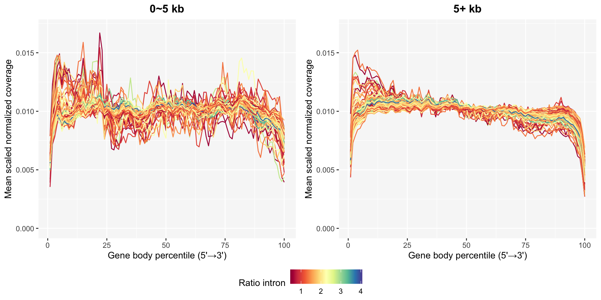

4.2 CVs per level

Metrics from scaled normalized transcript coverage for samples can be calculated by the get_metrics function. We employed sample level robustCV to compare trends with other sample properties and window CV matrix in a heatmap.

met = get_metrics(pileupPath, geneNames=genelist, rnum=100, method=1, scale=TRUE, margin=1)

head(round(met, 4))

##                     mean     sd     CV median    mad robustCV
## S000004-37958-003 0.0103 0.0033 0.3156 0.0105 0.0031   0.2957
## S000004-38071-002 0.0104 0.0032 0.3139 0.0106 0.0030   0.2886
## S000004-38094-003 0.0103 0.0033 0.3187 0.0105 0.0032   0.2998
## S000004-38120-002 0.0105 0.0035 0.3353 0.0107 0.0034   0.3165
## S000004-38134-002 0.0105 0.0035 0.3364 0.0106 0.0033   0.3130
## S000004-38138-003 0.0107 0.0039 0.3686 0.0108 0.0039   0.3580