5 Sample Quality
5.1 Sample quality index
A mean coverage depth (MCD) and a window coefficient of variation (wCV) can be calculated from the get_MCD and get_wCV functions.
Both functions return the same dimension of a matrix, which is (the number of genes) x (the number of samples).
MCD.mat = get_MCD(genelist, pileupPath, sampleInfo)
wCV.mat = get_wCV(genelist, pileupPath, sampleInfo, rnum=100, method=1, winSize=20, egPct=10)
dim(MCD.mat); dim(wCV.mat)
## [1] 1000 171## [1] 1000 171The get_SQI function gives the AUC of the fitted lines in the regression of wCV and log transformed MCD, and normalizes it using projection depth (PD)1.
Finally, we can determine the quality of the samples by defining them as Bad if they have PD> 3. Nineteen out of 171 samples are classified as bad quality samples.
The SQI plot shows the distribution of AUC and PD and the shape of the regression by sample quality.
result = get_SQI(MCD=MCD.mat, wCV=wCV.mat, rstPct=20, obsPct=50)

auc.vec <- result$auc.vec
table(auc.vec$SQI)
##
## Bad Good
## 19 152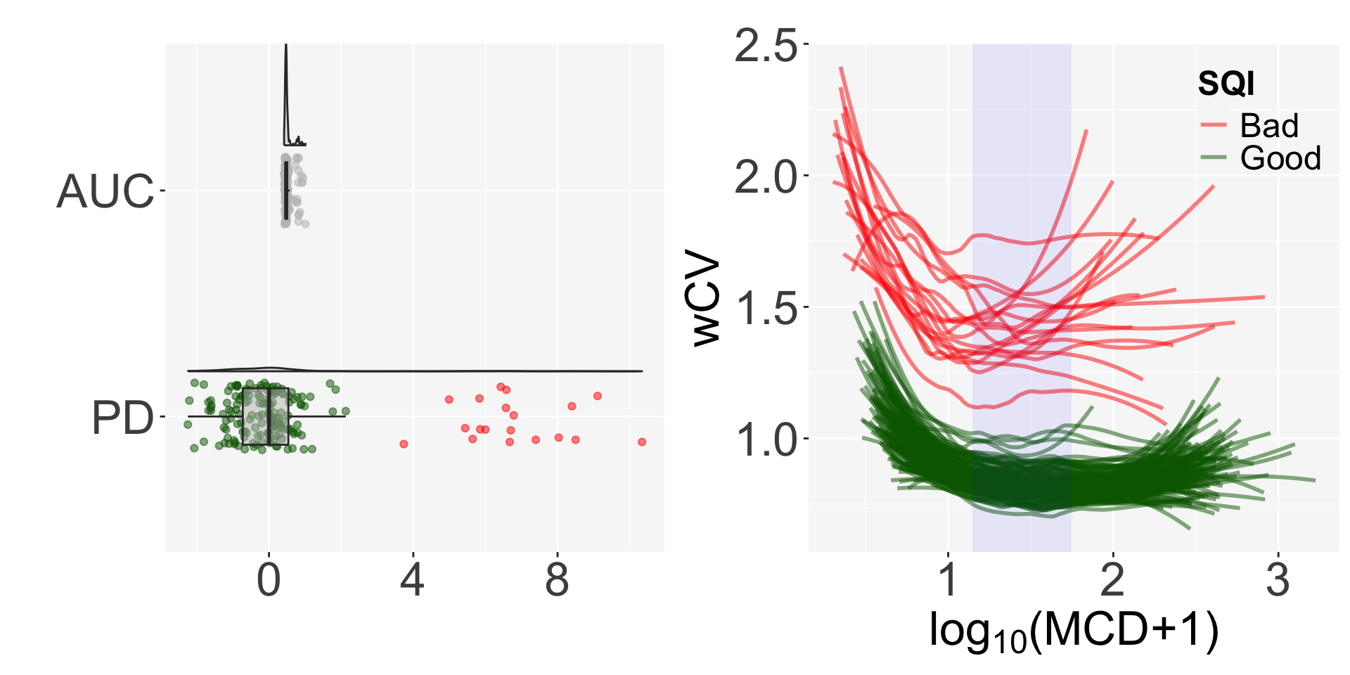
5.2 Updated gene body coverage
The gene body coverage plot can be updated after removing bad samples using the plot_GBCg function. The coverage patterns become much more stable, especially in the long genes.
A continuous legend can be selected among ratio intron and PD for the plot.
GBCg0 = plot_GBCg(stat=2, plot=TRUE, sampleInfo, GBCresult=GBC0, auc.vec=result$auc.vec)
GBCg5 = plot_GBCg(stat=2, plot=TRUE, sampleInfo, GBCresult=GBC5, auc.vec=result$auc.vec)

pg0 <- GBCg0$plotRI +
  coord_cartesian(ylim=c(0, 0.017)) +
  ggtitle("0~5 kb")

pg5 <- GBCg5$plotRI +
  coord_cartesian(ylim=c(0, 0.017)) +
  ggtitle("5+ kb")

ggpubr::ggarrange(pg0, pg5, common.legend=TRUE, legend="bottom", nrow=1)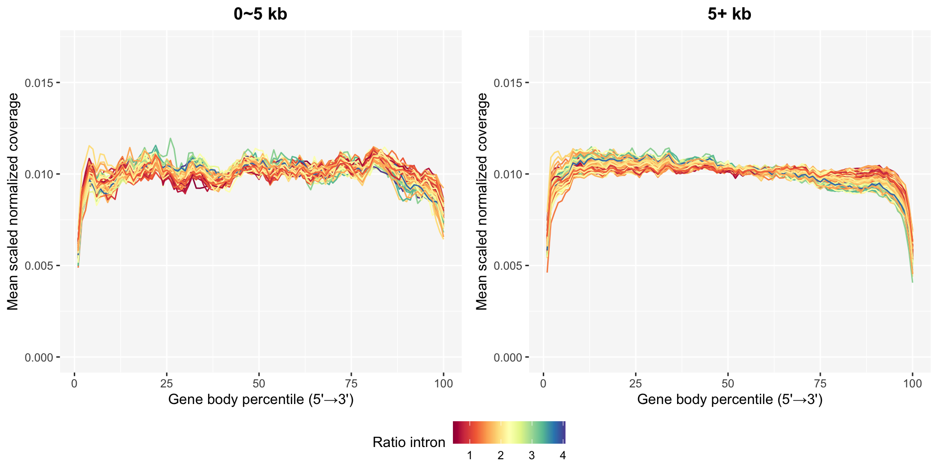
pg0 <- GBCg0$plotPD +
  coord_cartesian(ylim=c(0, 0.017)) +
  ggtitle("0~5 kb")

pg5 <- GBCg5$plotPD +
  coord_cartesian(ylim=c(0, 0.017)) +
  ggtitle("5+ kb")

ggpubr::ggarrange(pg0, pg5, common.legend=TRUE, legend="bottom", nrow=1)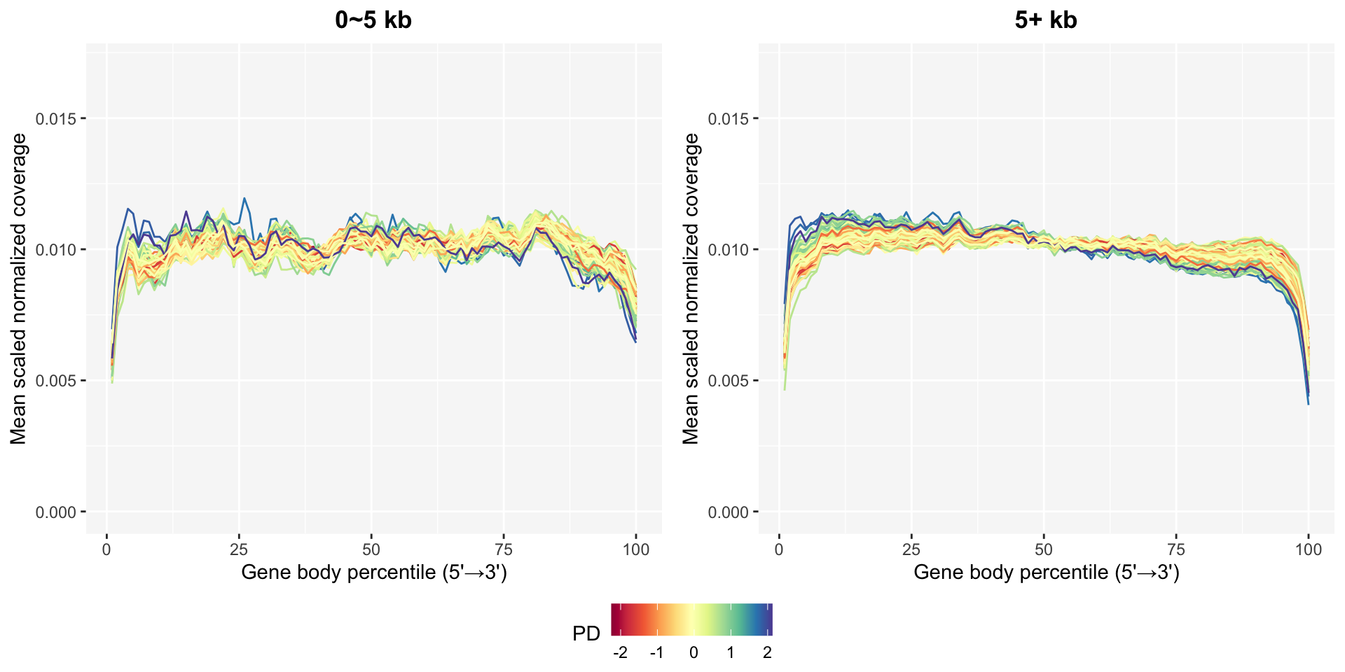
Choi, H. (2018). Scissor for finding outliers in RNA-seq. https://doi.org/10.17615/dv2e-7a29↩︎