Introduction to Continuous Time Markov Chains

from symbulate import *

from matplotlib import pyplot as plt

Seagull

Q = [[-1, 0.4, 0.6],
     [0.8 / 3,  -1 / 3, 0.2 / 3],
     [0.9 / 5, 0.1 / 5,  -1 / 5]]

pi0 = [1, 0, 0]

states = [1, 2, 3]

X = ContinuousTimeMarkovChain(Q, pi0, states)

plt.figure();
X.sim(1).plot()
plt.show();

plt.figure();
X.sim(3).plot()
plt.show();

plt.figure();
X[1 / 60].sim(10000).plot()
plt.show();

plt.figure();
X[0.5].sim(10000).plot()
plt.show();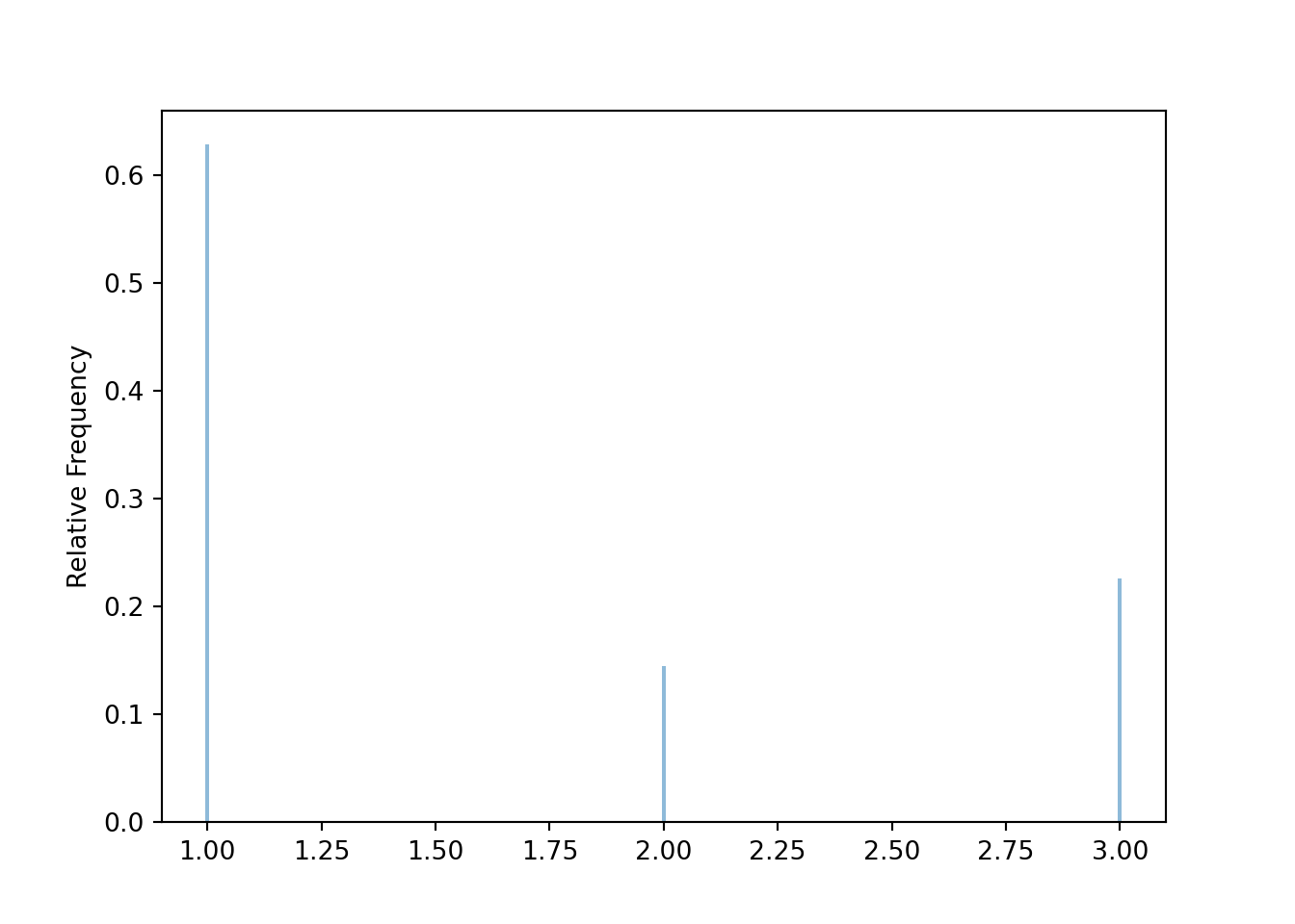

plt.figure();
X[1].sim(10000).plot()
plt.show();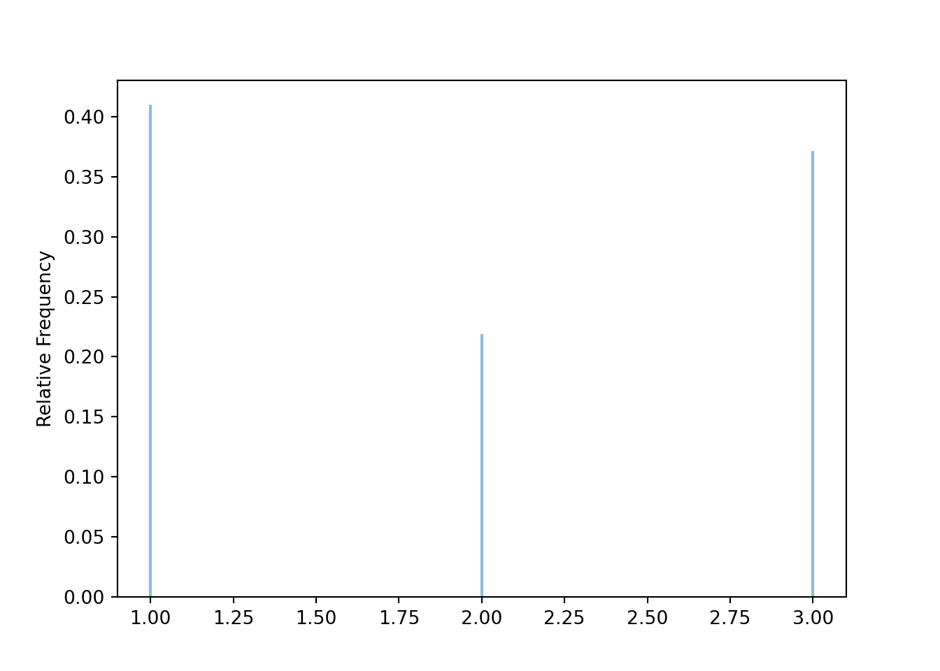

plt.figure();
X[5].sim(10000).plot()
plt.show();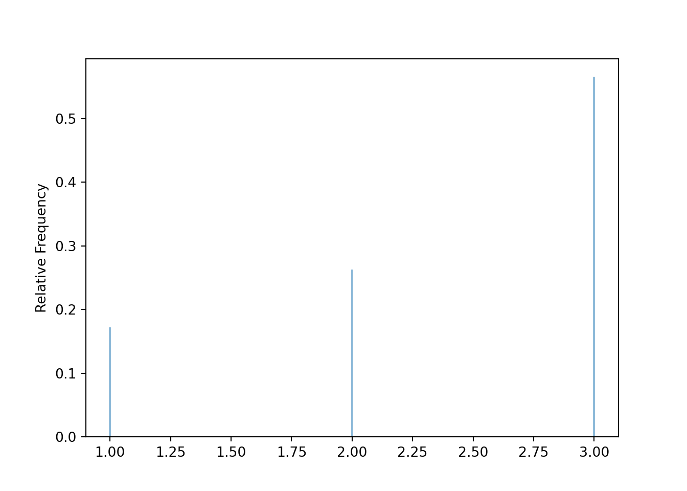

plt.figure();
X[60].sim(10000).plot()
plt.show();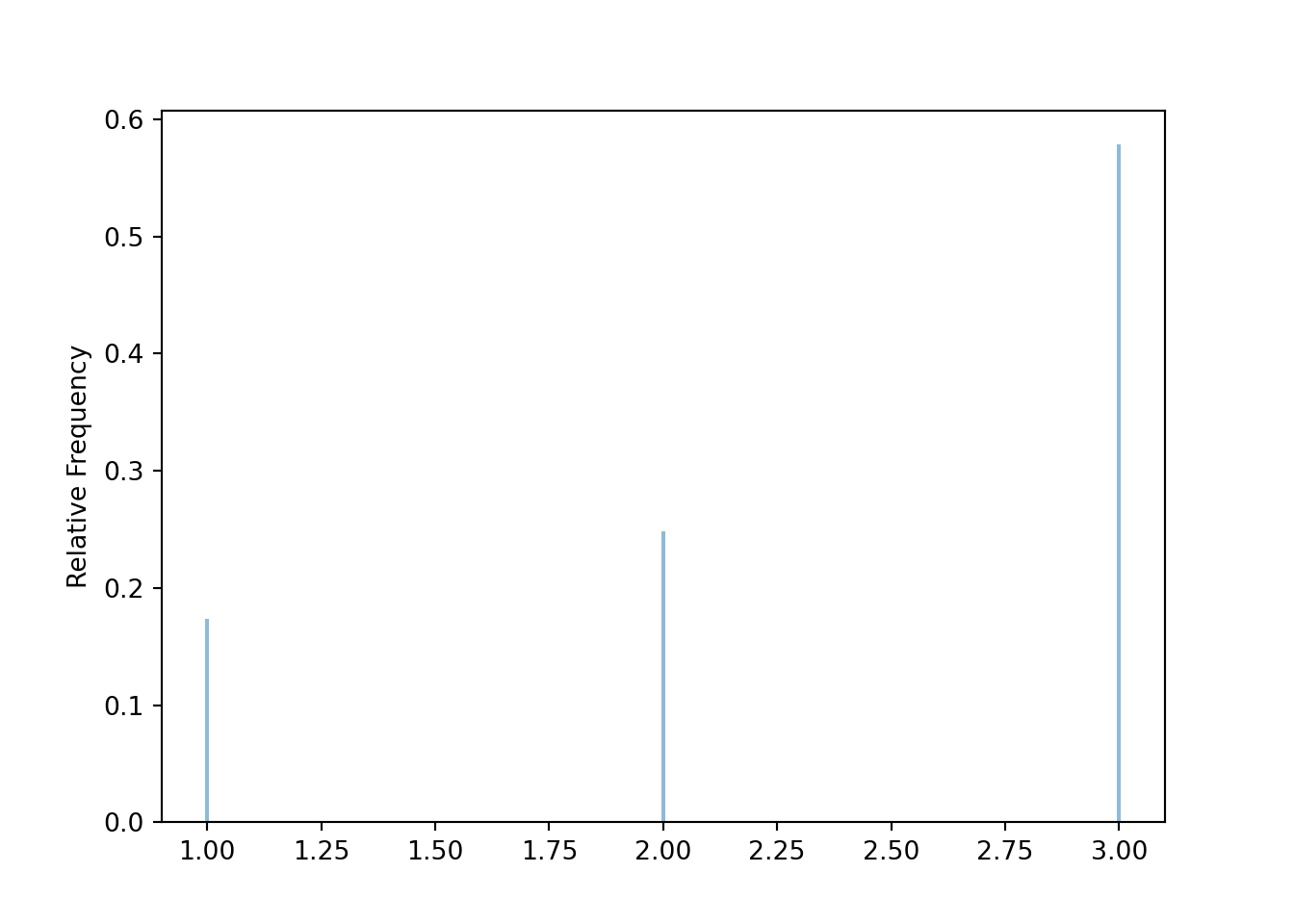

Times between jumps

P = ContinuousTimeMarkovChainProbabilitySpace(Q, pi0, states)
W = RV(P, interarrival_times)

plt.figure();
W[0].sim(10000).plot()
plt.show();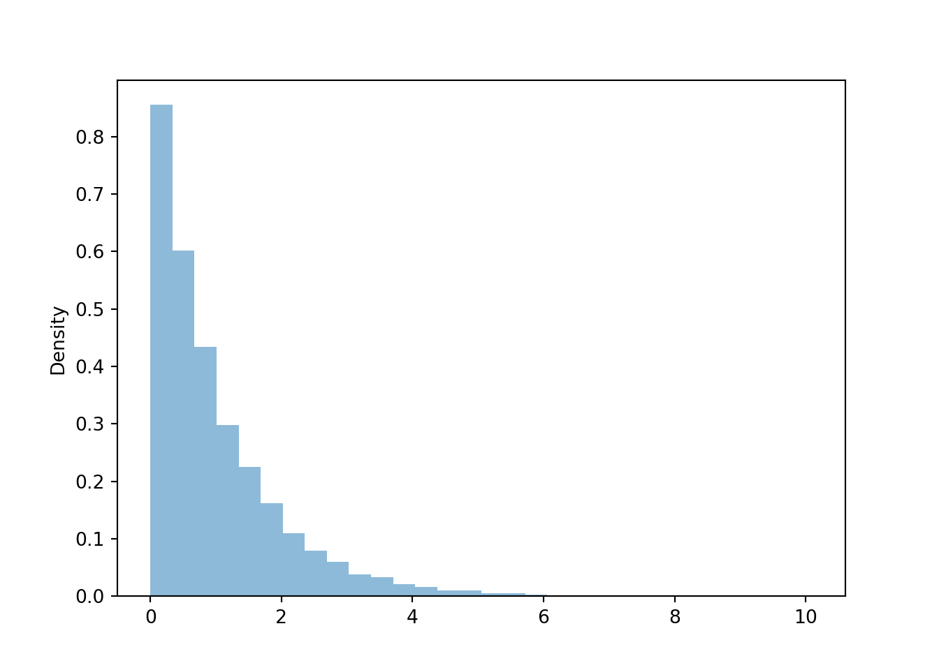

plt.figure();
W[1].sim(10000).plot()
plt.show();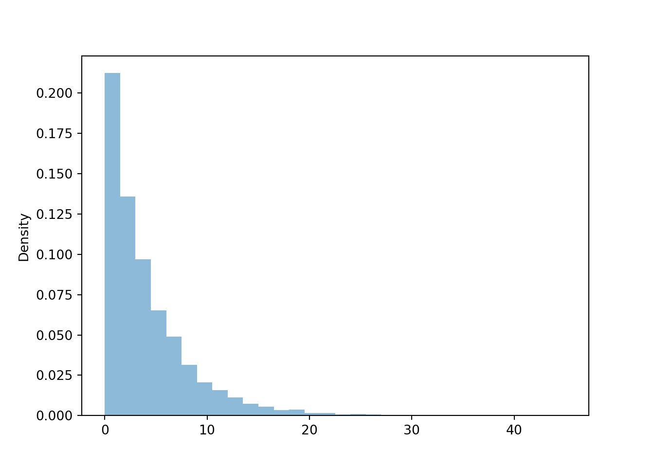

plt.figure();
(W[0] & W[1]).sim(10000).plot()
plt.show();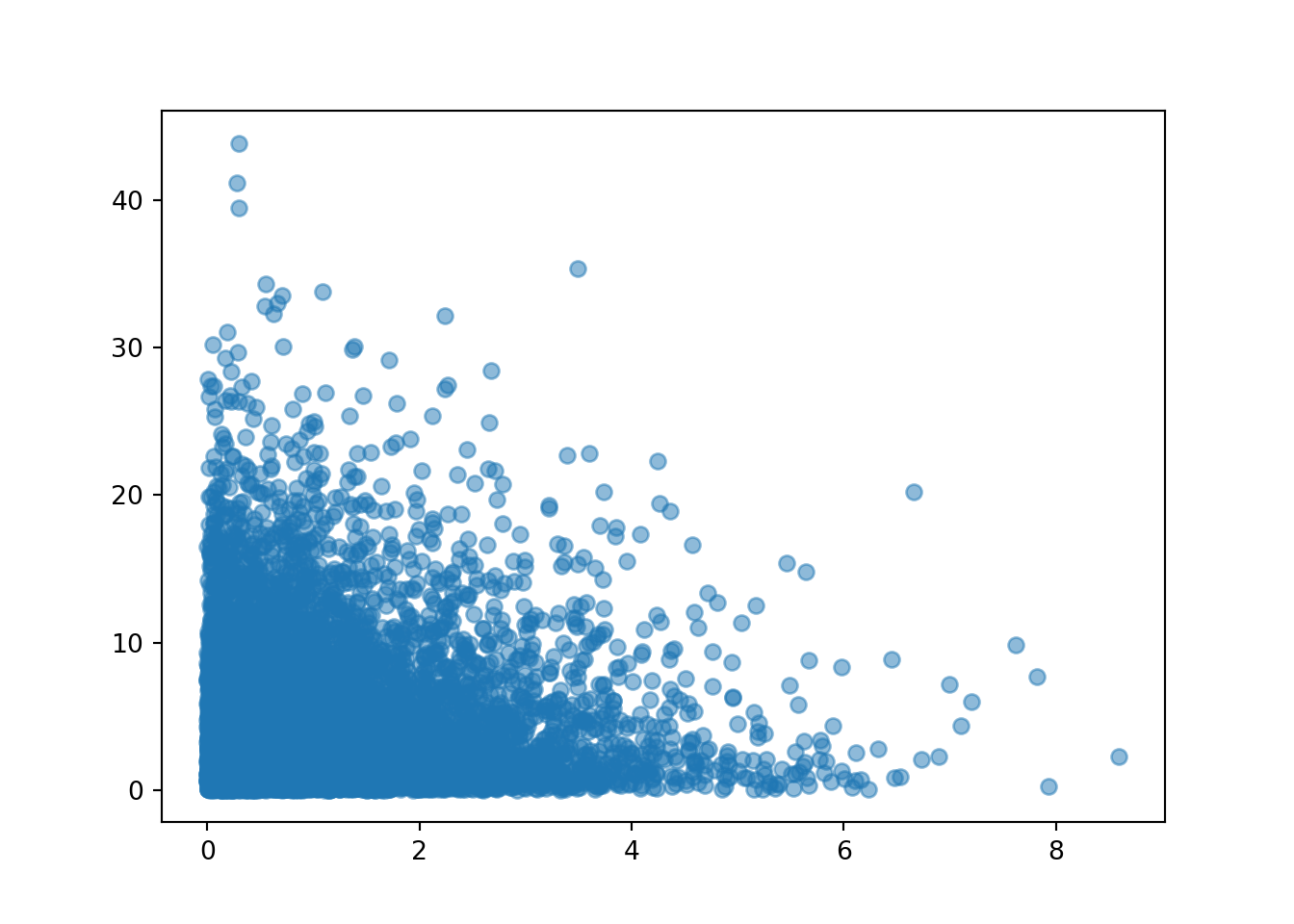

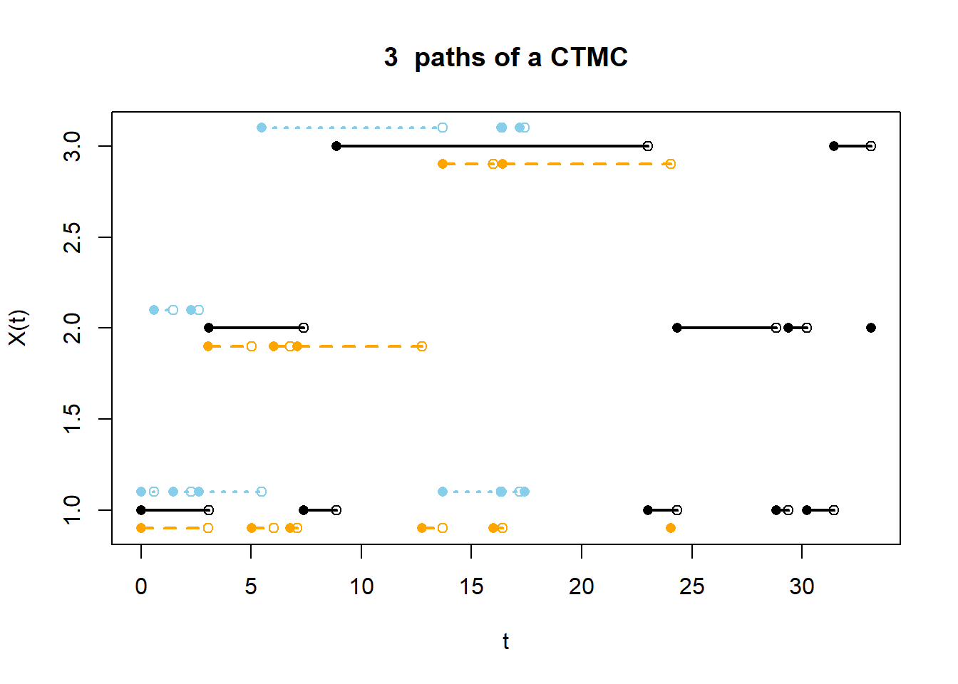
A few paths from scratch

states = 1:3 # state space

pi0 = c(1, 0, 0) # initial distribution

P = rbind(
  c(0, 0.6, 0.4),
  c(0.8, 0, 0.2),
  c(0.9, 0.1, 0)
) # transition matrix of embedded DTMC

lambda = c(1, 1 / 3, 1 / 5)  # transition rates for each state

Nruns = 3 # number of paths to simulate
Njump = 10  # number of transitions to sim for each path

Xt = matrix(rep(NA, Nruns * (Njump + 1)), nrow = Njump + 1) # +1 to include time 0
Wn = Xt


for (r in 1:Nruns){
  Xt[1, r] = sample(states, 1, prob = pi0) # initial state
  Wn[1, r] = 0 # time 0
  for (n in 2:(Njump+1)){
    Tn = rexp(1) / lambda[Xt[n - 1, r]] # time between jumps, exp(lambda_i)
    Xt[n, r] = sample(states, 1, prob = P[Xt[n - 1, r], ]) # new state
    Wn[n,r] = Wn[n - 1, r] + Tn # time of nth jump
  }
}
# Plot the paths
Npaths = Nruns
plotadj = c(0, -.1, .1)
plot(range(Wn),
     range(states)+range(plotadj),
     type = 'n',
     ylab = "X(t)", xlab = "t",
     main = paste(Npaths," paths of a CTMC"))
colors = c("black","orange","skyblue")

for (r in 1:Npaths){
  segments(y0 = Xt[-(Njump + 1), r] + plotadj[r],
           x0 = Wn[-(Njump + 1), r],
           y1 = Xt[-(Njump + 1), r] + plotadj[r],
           x1 = Wn[-1, r], col = colors[r], lty = r, lwd = 2)
  points(Wn[, r], Xt[,r] + plotadj[r], pch = 16, col = colors[r])
  points(Wn[-1, r], Xt[-(Njump + 1), r] + plotadj[r], col = colors[r])
}

M/M/1 Queue: Sample Path

lambda = 0.2

mu = 0.5

n_jumps = 20

X_t = rep(NA, n_jumps + 1)
T_n = rep(NA, n_jumps + 1)

X_t[1] = 0
T_n[1] = 0

for (n in 2:n_jumps){
  if (X_t[n - 1] == 0){
    T_n[n] = T_n[n - 1] + rexp(1) / lambda
    X_t[n] = X_t[n - 1] + 1
  } else {
    T_n[n] = T_n[n - 1] + rexp(1) / (lambda + mu)
    X_t[n] = X_t[n - 1] + sample(c(-1, 1), 1, prob = c(mu, lambda))
  }
}

plot(T_n, X_t,
     type = "s",
     xlab = "t", ylab = "X(t)",
     main = "Sample path of M/M/1 queue")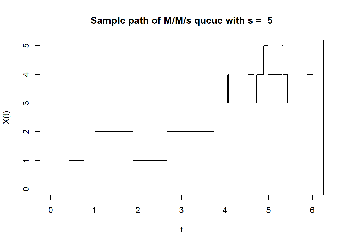

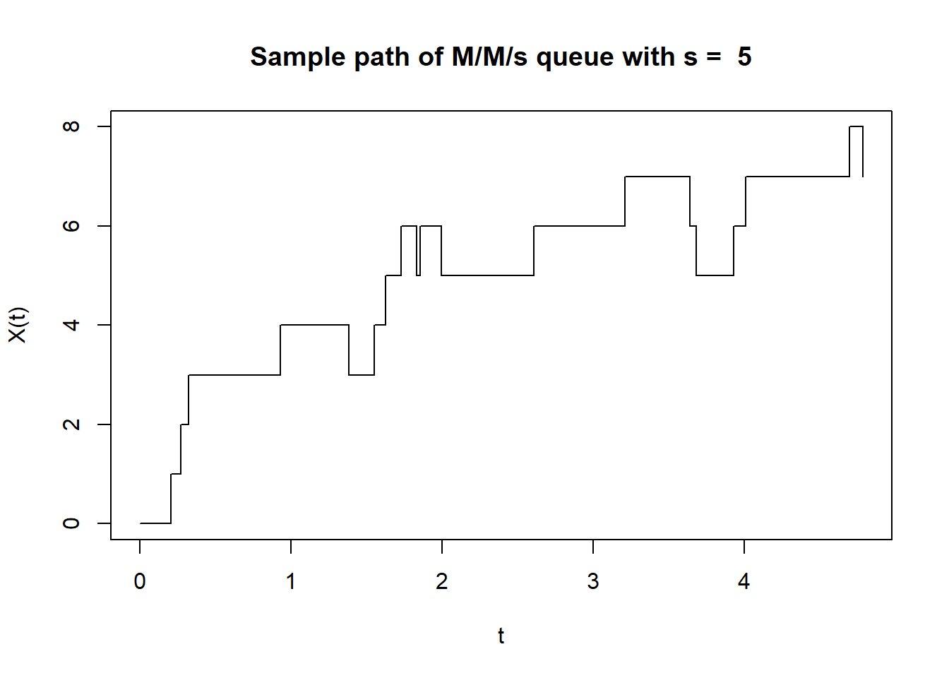
M/M/s Queue: Sample path

lambda = 2.3

mu = 0.5

s = 5
  
n_jumps = 20

X_t = rep(NA, n_jumps + 1)
W_n = rep(NA, n_jumps + 1)

X_t[1] = 0
W_n[1] = 0

for (n in 2:n_jumps){
    W_n[n] = W_n[n - 1] + rexp(1) / (lambda + mu * min(s, X_t[n - 1]))
    X_t[n] = X_t[n - 1] + sample(c(-1, 1), 1,
                                 prob = c(mu * min(s, X_t[n - 1]), lambda))
}

plot(W_n, X_t,
     type = "s",
     xlab = "t", ylab = "X(t)",
     main = paste("Sample path of M/M/s queue with s = ", s))