x_obs = c(1, 1, 2, 2, 2, 1, 2, 1, 2, 2, 2, 1, 2, 2, 1, 2, 2, 2, 1, 1, 2)

table(x_obs, lead(x_obs, 1))
x_obs 1 2
    1 2 6
2 5 7x_obs = c(1, 1, 2, 2, 2, 1, 2, 1, 2, 2, 2, 1, 2, 2, 1, 2, 2, 2, 1, 1, 2)
table(x_obs, lead(x_obs, 1))
x_obs 1 2
1 2 6
2 5 7I couldn’t find Markov’s actual sequence data, so I created a sequence of states that matches his pair counts.
markov_letter_sequence = read_csv("markov_letter_data.csv")

head(markov_letter_sequence)
# A tibble: 6 × 2
time state
<dbl> <dbl>
1 0 2
2 1 1
3 2 1
4 3 1
5 4 1
6 5 1x_obs = markov_letter_sequence$state
table(x_obs, lead(x_obs, 1))
x_obs    1    2
    1 1104 7534
    2 7535 3827
Using the markovchain package.
library(markovchain)mc_fit = markovchainFit(data = x_obs, method = "mle")
mc_fit$estimate
MLE Fit
A 2 - dimensional discrete Markov Chain defined by the following states:
1, 2
The transition matrix (by rows) is defined as follows:
1 2
1 0.1278074 0.8721926
2 0.6631755 0.3368245
$standardError
1 2
1 0.003846550 0.010048462
2 0.007639885 0.005444706
$confidenceLevel
[1] 0.95
$lowerEndpointMatrix
1 2
1 0.1202683 0.8524980
2 0.6482016 0.3261531
$upperEndpointMatrix
1 2
1 0.1353465 0.8918873
2 0.6781494 0.3474959
$logLikelihood
[1] -10560.68createSequenceMatrix(x_obs) 1 2
1 1104 7534
2 7535 3827These confidence intervals adjust for the correlation
multinomialConfidenceIntervals(transitionMatrix =
                                 mc_fit$estimate@transitionMatrix,
                               countsTransitionMatrix = createSequenceMatrix(x_obs))
$confidenceLevel
[1] 0.95
$lowerEndpointMatrix
1 2
1 0.1209771 0.8653624
2 0.6541982 0.3278472
$upperEndpointMatrix
1 2
1 0.1348674 0.8792526
2 0.6722571 0.3459061state_names = c("v", "c")
P = rbind(
c(0.128, 0.872),
c(0.663, 0.337)
)
pi_0 = c(0.432, 0.568)x_current = factor(simulate_single_DTMC_path(c(1, 0), P, 50000))
head(x_current, 10) [1] 1 2 1 2 1 2 1 2 1 2
Levels: 1 2createSequenceMatrix(x_current) 1 2
1 2653 18883
2 18882 9582mc_fit = markovchainFit(data = x_current, method = "mle")
mc_fit$estimate
MLE Fit
A 2 - dimensional discrete Markov Chain defined by the following states:
1, 2
The transition matrix (by rows) is defined as follows:
1 2
1 0.1231891 0.8768109
2 0.6633642 0.3366358
$standardError
1 2
1 0.002391683 0.006380731
2 0.004827564 0.003439000
$confidenceLevel
[1] 0.95
$lowerEndpointMatrix
1 2
1 0.1185015 0.8643049
2 0.6539024 0.3298954
$upperEndpointMatrix
1 2
1 0.1278767 0.8893169
2 0.6728261 0.3433761
$logLikelihood
[1] -26220.11The verifyMarkovProperty function conduct a goodness of fit hypothesis test to see if a sequence follows a Markov chain. The null hypothesis is that the sequence is generated from a MC. If the p-value is small there is evidence that the Markov assumption is NOT reasonable.
verifyMarkovProperty(x_current)Testing markovianity property on given data sequence
Chi - square statistic is: 0.4005617
Degrees of freedom are: 5
And corresponding p-value is: 0.9953141 Now we’ll summarize the data ourselves. First we’ll create columns for the current state, next state, and previous state.
x = tibble(x_current,
x_next = lead(x_current, 1),
x_previous = lag(x_current, 1))
x |> head()# A tibble: 6 × 3
x_current x_next x_previous
<fct> <fct> <fct>
1 1 2 <NA>
2 2 1 1
3 1 2 2
4 2 1 1
5 1 2 2
6 2 1 1 Now we’ll tabulate the (current state, next state) pairs using both base R and tidyverse.
table(x$x_current, x$x_next)
      1     2
1  2653 18883
2 18882 9582x_summary = x |>
group_by(x_current) |>
count(x_next, name = "count") |>
filter(!is.na(x_next))
x_summary |> kbl() |> kable_styling()| x_current | x_next | count |
|---|---|---|
| 1 | 1 | 2653 |
| 1 | 2 | 18883 |
| 2 | 1 | 18882 |
| 2 | 2 | 9582 |
Now we can use the tabulated data to create a bar plot of the conditional distributions of the next state given each current state. (We’ll use ggplot.)
x_summary |>
  ggplot(aes(x = x_current,
             y = count,
             fill = x_next)) +
  geom_bar(position = "fill",
           stat = "identity") +
  scale_fill_viridis_d() +
  labs(y = "Conditional probability given current state")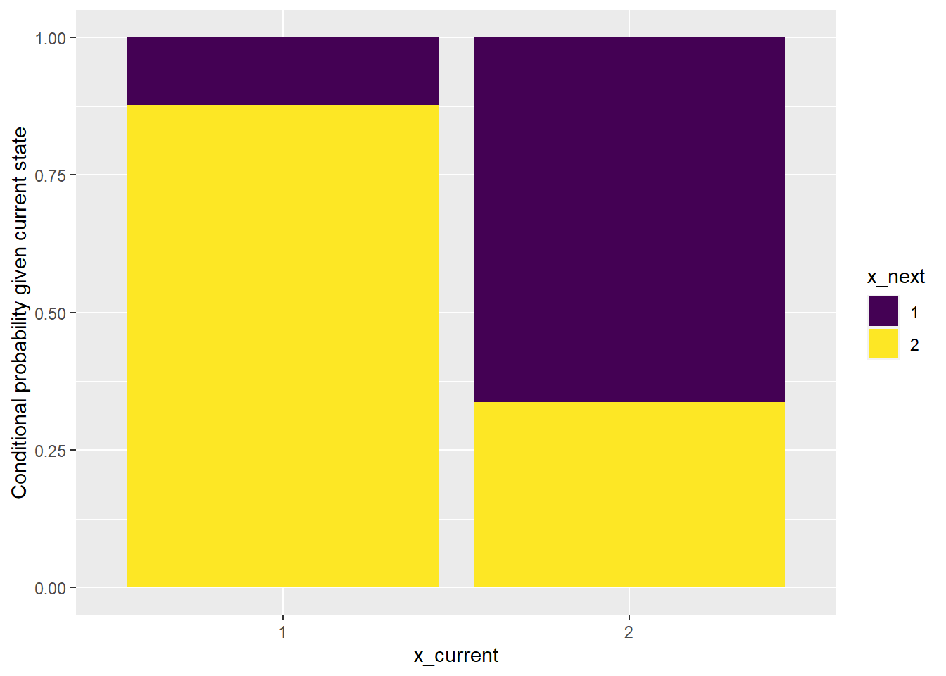
The bar plot above shows that it would not be reasonable to consider the data as being generated by an independent sequence.
Now we’ll create a plot to assess if the Markov assumption is reasonable. To do so we need to check if the next state and previous state are conditionally indepdent given the current state.
First we tabulate the (x_previous, x_current, x_next) triples.
Using base R table, if you put x_current last it will create tables of (x_previous, x_next) for each value of x_current.
table(x$x_previous, x$x_next, x$x_current), , = 1
1 2
1 331 2322
2 2322 16560
, , = 2
1 2
1 12548 6335
2 6334 3247x_summary_mc = x |>
group_by(x_current, x_previous) |>
count(x_next, name = "count") |>
filter(!is.na(x_next) & !is.na(x_previous))
x_summary_mc |> kbl() |> kable_styling()| x_current | x_previous | x_next | count |
|---|---|---|---|
| 1 | 1 | 1 | 331 |
| 1 | 1 | 2 | 2322 |
| 1 | 2 | 1 | 2322 |
| 1 | 2 | 2 | 16560 |
| 2 | 1 | 1 | 12548 |
| 2 | 1 | 2 | 6335 |
| 2 | 2 | 1 | 6334 |
| 2 | 2 | 2 | 3247 |
Now we can use the tabulated data to create a bar plot of the conditional distributions of the next state given each previous state, further conditioned on each current state (using facets). (We’ll use ggplot.)
x_summary_mc |>
  ggplot(aes(x = x_previous,
             y = count,
             fill = x_next)) +
  geom_bar(position = "fill",
           stat = "identity") +
  scale_fill_viridis_d() +
  labs(y = "Conditional probability given previous state") +
  facet_wrap(~x_current, labeller = label_both)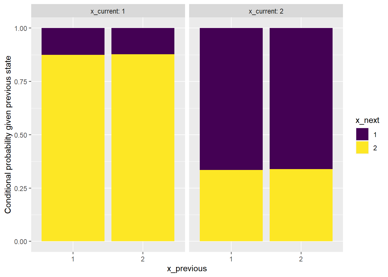
The plot shows that it is reasonable to consider the sequence as being generated from a Markov chain.
state_names = c("RR", "NR", "RN", "NN")

P = rbind(c(.7, 0, .3, 0),
          c(.5, 0, .5, 0),
          c(0, .4, 0, .6),
          c(0, .2, 0, .8)
)

x_obs = simulate_single_DTMC_path(c(1, 0, 0, 0), P, 100000)

x_current = str_sub(state_names[x_obs], start = 1, end = 1)

x_current |> head()
[1] "R" "R" "R" "N" "N" "N"x = tibble(x_current,
x_next = lead(x_current, 1),
x_previous = lag(x_current, 1))
x |> head()# A tibble: 6 × 3
x_current x_next x_previous
<chr> <chr> <chr>
1 R R <NA>
2 R R R
3 R N R
4 N N R
5 N N N
6 N N N x_summary_mc = x |>
group_by(x_current, x_previous) |>
count(x_next, name = "count") |>
filter(!is.na(x_next) & !is.na(x_previous))
x_summary_mc |> kbl() |> kable_styling()| x_current | x_previous | x_next | count |
|---|---|---|---|
| N | N | N | 36539 |
| N | N | R | 8981 |
| N | R | N | 8982 |
| N | R | R | 5978 |
| R | N | N | 7588 |
| R | N | R | 7371 |
| R | R | N | 7372 |
| R | R | R | 17188 |
x_summary_mc |>
  ggplot(aes(x = x_previous,
             y = count,
             fill = x_next)) +
  geom_bar(position = "fill",
           stat = "identity") +
  scale_fill_viridis_d() +
  labs(y = "Conditional probability given previous state") +
  facet_wrap(~x_current, labeller = label_both)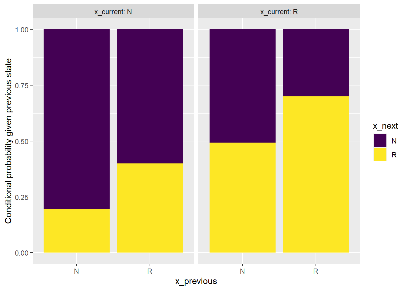
From the bar plot we can see that the sequence can NOT be considered to be generated from a first order Markov chain.
Here is a test; note the small p-value (recall that the null hypothesis is a MC model).
verifyMarkovProperty(x_current)Testing markovianity property on given data sequence
Chi - square statistic is: 4169.859
Degrees of freedom are: 5
And corresponding p-value is: 0 To see if
Note: we actually simulated this sequence by simulating the
x_and_y = x |>
  filter(!is.na(x_next) & !is.na(x_previous)) |>
  unite("y_current", c("x_previous", "x_current"), remove = FALSE) |>
  mutate(y_next = lead(y_current, 1),
         y_previous = lag(y_current, 1))

x_and_y |> select(x_previous, x_current, y_current, y_previous, y_next) |> head()
# A tibble: 6 × 5
x_previous x_current y_current y_previous y_next
<chr> <chr> <chr> <chr> <chr>
1 R R R_R <NA> R_R
2 R R R_R R_R R_N
3 R N R_N R_R N_N
4 N N N_N R_N N_N
5 N N N_N N_N N_N
6 N N N_N N_N N_N We can assess if
y_summary_mc = x_and_y |>
  group_by(y_current, y_previous) |>
  count(y_next, name = "count") |>
  filter(!is.na(y_next) & !is.na(y_previous))

y_summary_mc |> kbl() |> kable_styling()| y_current | y_previous | y_next | count |
|---|---|---|---|
| N_N | N_N | N_N | 29340 |
| N_N | N_N | N_R | 7197 |
| N_N | R_N | N_N | 7198 |
| N_N | R_N | N_R | 1784 |
| N_R | N_N | R_N | 4594 |
| N_R | N_N | R_R | 4387 |
| N_R | R_N | R_N | 2994 |
| N_R | R_N | R_R | 2984 |
| R_N | N_R | N_N | 4563 |
| R_N | N_R | N_R | 3025 |
| R_N | R_R | N_N | 4419 |
| R_N | R_R | N_R | 2953 |
| R_R | N_R | R_N | 2244 |
| R_R | N_R | R_R | 5127 |
| R_R | R_R | R_N | 5128 |
| R_R | R_R | R_R | 12060 |
y_summary_mc |>
  ggplot(aes(x = y_previous,
             y = count,
             fill = y_next)) +
  geom_bar(position = "fill",
           stat = "identity") +
  scale_fill_viridis_d() +
  labs(y = "Conditional probability given previous state") +
  facet_wrap(~y_current, labeller = label_both)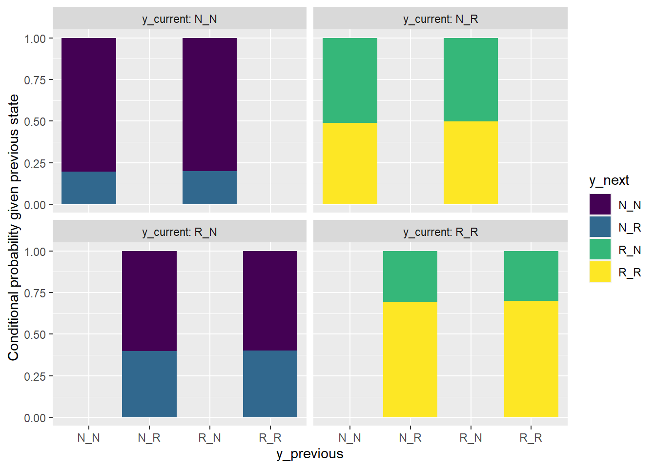
The bar plot shows that it is reasonable to consider
verifyMarkovProperty(x_and_y$y_current)Testing markovianity property on given data sequence
Chi - square statistic is: 2.730365
Degrees of freedom are: 11
And corresponding p-value is: 0.9938309