Introduction to Stochastic Processes
A stochastic process \(X(t)\) is defined by \[ X(t) = A+Bt, \qquad t\ge0 \] where \(A\) and \(B\) are discrete random variables with joint pmf
b | ||
a | 0 | 1 |
0 | 0.1 | 0.3 |
2 | 0.2 | 0.4 |
Note: this process is unlike most of the processes we’ll study in that all of the randomness in this process is resolved at time 0, while most of the processes we’ll study will truly experience randomness over time. But this process gives you an example where you can explicitly draw some sample paths as simple functions of time.
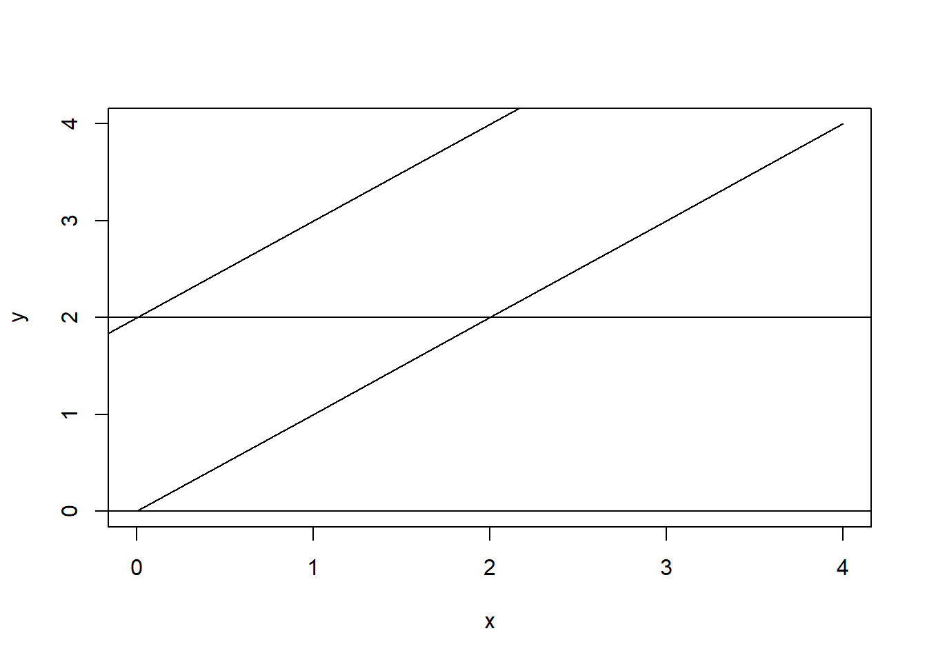
- Draw a plot of all possible sample paths of this stochastic process. Your plot should be well drawn with well labeled axes.
- Is \(X(t)\) a discrete or continuous time process?
- Continuous time process because the index set for time is uncountable.
- Is \(X(t)\) a discrete or continuous state process?
- Continuous state process because the index set for state is uncountable.
- Specify the joint distribution of \(X(2)\) and \(X(3)\).
(X=2,X=3) | |
---|---|
(0,0) | 0.1 |
(2,2) | 0.2 |
(2,3) | 0.3 |
(4,5) | 0.4 |
- Specify the distribution of \(X(2)\).
(X=2) | |
---|---|
0 | 0.1 |
2 | 0.5 |
4 | 0.4 |
- Compute \(\text{E}(X(2))\).
\(\text{E}(X(2))=0(0.1)+2(0.5)+4(0.4)\)
\(\text{E}(X(2))=2.6\)
- Compute \(\text{Var}(X(2))\).
\(\text{Var}(X(2))=0(0.1-2.6)^2+0.3(2-2.6)^2+0.2(2-2.6)^2+0.4(4-2.6)^2\)
\(\text{Var}(X(2))=1.64\)
- Specify the distribution of \(X(3)\).
(X=3) | |
---|---|
0 | 0.1 |
2 | 0.2 |
3 | 0.3 |
5 | 0.4 |
- Compute \(\text{E}(X(3))\).
\(\text{E}(X(3))=0(0.1)+2(0.2)+3(0.3)+5(0.4)\)
\(\text{E}(X(3))=3.3\)
- Compute \(\text{Var}(X(3))\).
\(\text{Var}(X(3))=0.1(0-3.3)^2+0.2(2-3.3)^2+0.3(3-3.3)^2+0.4(5-3.3)^2\)
\(\text{Var}(X(3))=2.61\)
- Compute \(\text{Cov}(X(2), X(3))\).
\(\text{Cov}(X(2), X(3))={E}(X(2)X(3))-{E}(X(2)){E}(X(3))\)
\(\text{Cov}(X(2), X(3))=(0)(0)(0.1)+(2)(3)(0.3)+(2)(2)(0.2)+(4)(5)(0.4)-(2.6)(3.3)\)
\(\text{Cov}(X(2), X(3))=2.02\)
- Find an expression for \(\text{E}(X(t))\) as a function of \(t\) (this is called the mean function of \(X(t)\)).
\(\text{E}(X(t))=0(0.4)+2(0.6)+0(0.3)t+1(0.7)t\)
\(\text{E}(X(t))=1.2+0.7t\)
- Find an expression for \(\text{Var}(X(t))\) as a function of \(t\) (this is called the variance function of \(X(t)\)).
\(\text{Var}(X(t))={Var}(A+Bt)\)
\(\text{Var}(A+Bt)={Var}(A)+t^2{Var}(B)+2t{Cov}(A,B)\)
\(\text{Var}(A)={E}(A^2)-{E}(A)^2\)
\(\text{Var}(A)=4(0.6)-(2(0.6))^2\)
\(\text{Var}(A)=0.96\)
\(\text{Var}(B)=t^2[{E}(B^2)-{E}(B)^2]\)
\(\text{Var}(B)=1(0.7)-(1(0.7))^2\)
\(\text{Var}(B)=0.21\)
\(\text{Cov}(A,B)={E}(AB)-{E}(A){E}(B)\)
\(\text{Cov}(A,B)= 0.8-((1.2)(0.7))\)
\(\text{Cov}(A,B)=-0.4\)
\(\text{Var}(A+Bt)={Var}(A)+t^2{Var}(B)+2t{Cov}(A,B)\)
\(\text{Var}(A+Bt)=0.96+t^2(0.21)+2t(-0.4)\)
\(\text{Var}(A+Bt)=0.96-0.8t+0.21t^2\)