mean_time_to_absorption <- function(transition_matrix, state_names = NULL) {

  absorbing_states = which(diag(transition_matrix) == 1)

  if (length(absorbing_states) == 0) stop("There are no absorbing states.")

  n_states = nrow(transition_matrix)

  transient_states = setdiff(1:n_states, absorbing_states)

  Q = transition_matrix[transient_states, transient_states]

  mtta = solve(diag(nrow(Q)) - Q, rep(1, nrow(Q)))

  if (is.null(state_names)) state_names = 1:n_states

  data.frame(start_state = state_names[transient_states],
             mean_time_to_absorption = mtta)
}Absorbing States and First Step Analysis
Function to compute mean time to absorption for absorbing chain
This function basically just computes solve(I - Q, ones), but there’s some rearranging required to put the transition matrix in canonical form.
Function to compute pmf of time to absorption given the initial state.
pmf_of_time_to_absorption <- function(transition_matrix, state_names = NULL, start_state) {

  absorbing_states = which(diag(transition_matrix) == 1)

  if (length(absorbing_states) == 0) stop("There are no absorbing states.")

  n_states = nrow(transition_matrix)

  transient_states = setdiff(1:n_states, absorbing_states)

  if (is.null(state_names)) state_names = 1:n_states

  if (which(state_names == start_state) %in% absorbing_states) stop("Initial state is an absorbing state; absorption at time 0.")

  n = 1

  TTA_cdf = sum(transition_matrix[which(state_names == start_state), absorbing_states])

  while (max(TTA_cdf) < 0.999999) {

    n = n + 1

    TTA_cdf = c(TTA_cdf, sum((transition_matrix %^% n)[which(state_names == start_state), absorbing_states]))
  }

  TTA_pmf = TTA_cdf - c(0, TTA_cdf[-length(TTA_cdf)])

  data.frame(n = 1:length(TTA_pmf),
             prob_absorb_at_time_n = TTA_pmf)
}
Function to compute probabilities of absorption in each absorbing state
This function basically just computes solve(I - Q, R), but there’s some rearranging required to put the transition matrix in canonical form.
absorption_probability <- function(transition_matrix, state_names = NULL) {

  absorbing_states = which(diag(transition_matrix) == 1)

  if (length(absorbing_states) == 0) stop("There are no absorbing states.")

  n_states = nrow(transition_matrix)

  transient_states = setdiff(1:n_states, absorbing_states)

  Q = transition_matrix[transient_states, transient_states]

  R = transition_matrix[transient_states, absorbing_states]

  absorption_probability = solve(diag(nrow(Q)) - Q, R)

  if (is.null(state_names)) state_names = 1:n_states

  colnames(absorption_probability) = paste("prob_absorb_in_state_",
                                           state_names[absorbing_states], sep = "")

  data.frame(start_state = state_names[transient_states],
             absorption_probability)
}
Ehrenfest urn chain - time to absorption
M = 5

state_names = 0:M

P = rbind(
  c(5, 0, 0, 0, 0, 0),
  c(1, 0, 4, 0, 0, 0),
  c(0, 2, 0, 3, 0, 0),
  c(0, 0, 3, 0, 2, 0),
  c(0, 0, 0, 4, 0, 1),
  c(0, 0, 0, 0, 0, 5)
) / 5

pi0 = c(0, 0, 0, 1, 0, 0) # start in state 3plot_state_diagram(P, state_names)Joining with `by = join_by(prob)`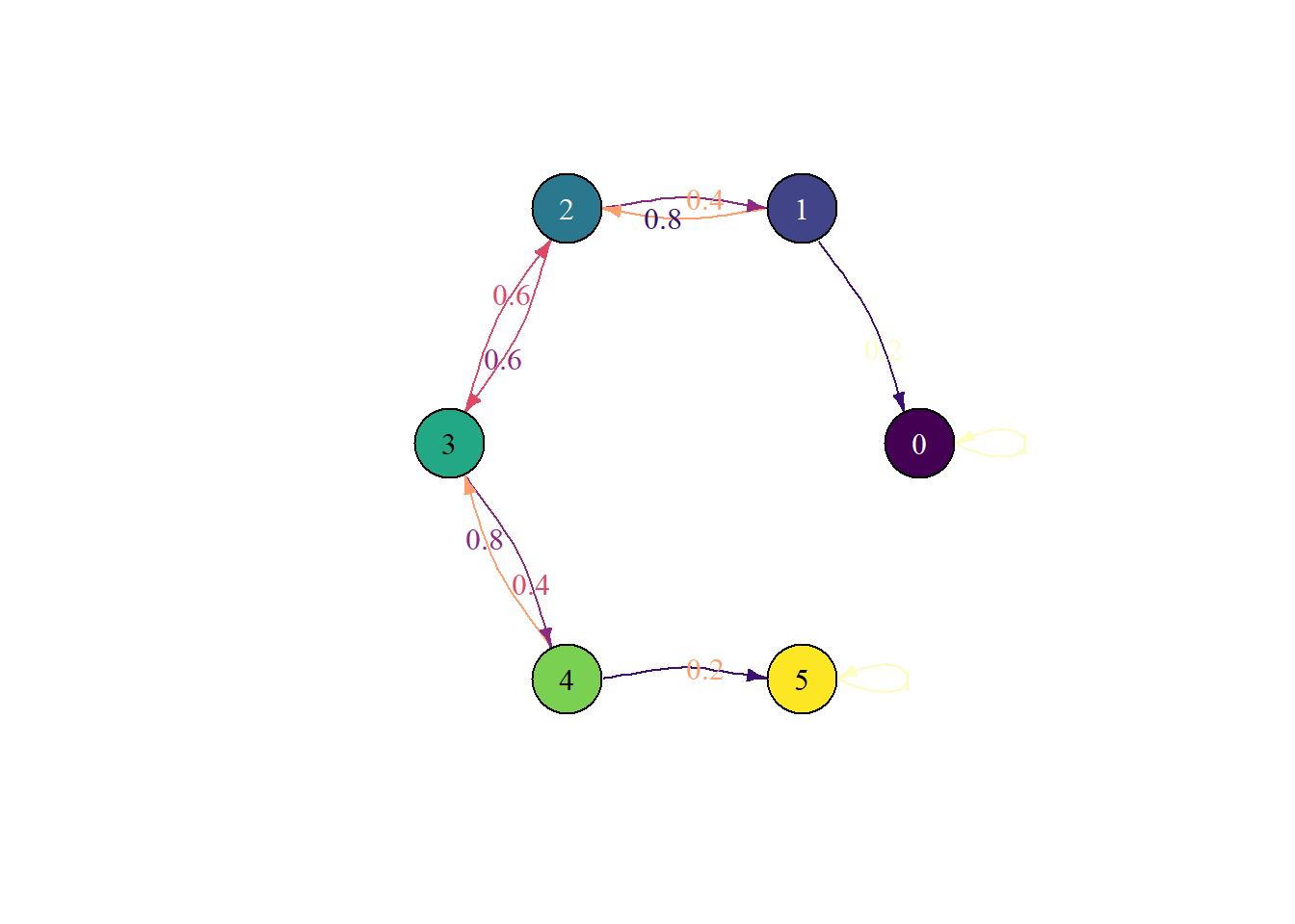
Simulation-based approximation of time to absorption
The simulate_DTMC_paths function reshapes the results from wide to long format for easier plotting. But it’s probably easier to leave in wide format - one row for each path - for the purposes of computing path random variables like time to absorption simulate_DTMC_paths function as is, which is why I’m running a loop below to simulate a single sample path, compute
Also, rather than running a while loop to stop at the first time of absorption, I’m just running a large number of steps (200) for each path and then finding what time absorption occurred.
absorbing_states = which(diag(P) == 1)

n_rep = 10000
time_to_absorption = rep(NA, n_rep)

for (i in 1:n_rep) {
  x = simulate_single_DTMC_path(pi0, P, last_time = 200)
  time_to_absorption[i] = min(which(x %in% absorbing_states))
}

hist(time_to_absorption)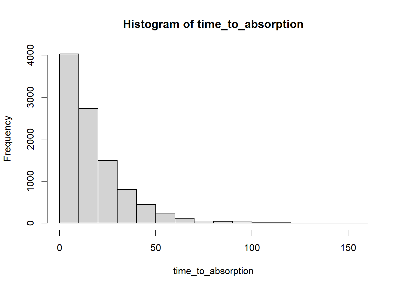
summary(time_to_absorption) Min. 1st Qu. Median Mean 3rd Qu. Max.
3.00 7.00 13.00 18.43 25.00 152.00 mean(time_to_absorption)[1] 18.4339sd(time_to_absorption)[1] 16.23996Mean time to absorption given each initial state
Q = P[2:5, 2:5]

Q
[,1] [,2] [,3] [,4]
[1,] 0.0 0.8 0.0 0.0
[2,] 0.4 0.0 0.6 0.0
[3,] 0.0 0.6 0.0 0.4
[4,] 0.0 0.0 0.8 0.0solve(diag(4) - Q, rep(1, 4))[1] 15.0 17.5 17.5 15.0Using the function
mtta = mean_time_to_absorption(P, state_names)

mtta |> kbl() |> kable_styling()| start_state | mean_time_to_absorption |
|---|---|
| 1 | 15.0 |
| 2 | 17.5 |
| 3 | 17.5 |
| 4 | 15.0 |
Molecules distributed at random (assuming it’s possible they could start in an absorbing state).
sum(dbinom(0:M, M, 0.5) * c(0, mtta[, 2], 0))[1] 15.625Computation of distribution of time to absorption
T_pmf = pmf_of_time_to_absorption(P, start_state = 3)

T_pmf |> head(10) |> kbl() |> kable_styling()| n | prob_absorb_at_time_n |
|---|---|
| 1 | 0.0000000 |
| 2 | 0.0800000 |
| 3 | 0.0480000 |
| 4 | 0.0544000 |
| 5 | 0.0480000 |
| 6 | 0.0462080 |
| 7 | 0.0430848 |
| 8 | 0.0406374 |
| 9 | 0.0381696 |
| 10 | 0.0359057 |
ggplot(T_pmf |>
         filter(prob_absorb_at_time_n > 0),
       aes(x = n,
           y = prob_absorb_at_time_n)) +
  geom_line(linewidth = 1)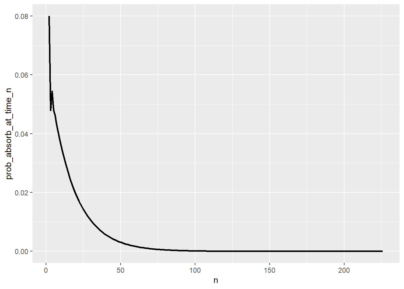
sum(T_pmf[, 1] * T_pmf[, 2])[1] 17.49977Rick rolls
States: 0 -> 1 -> 12 -> 123
Mean time to absorption
state_names = c("0", "1", "12", "123")

P = rbind(
  c(5, 1, 0, 0),
  c(4, 1, 1, 0),
  c(4, 1, 0, 1),
  c(0, 0, 0, 6)
  ) / 6

mean_time_to_absorption(P, state_names) |>
kbl() |> kable_styling()| start_state | mean_time_to_absorption |
|---|---|
| 0 | 216 |
| 1 | 210 |
| 12 | 180 |
Distribution of time to absorption
T_pmf = pmf_of_time_to_absorption(P, state_names, start_state = "0")

T_pmf |> head(10) |> kbl() |> kable_styling()| n | prob_absorb_at_time_n |
|---|---|
| 1 | 0.0000000 |
| 2 | 0.0000000 |
| 3 | 0.0046296 |
| 4 | 0.0046296 |
| 5 | 0.0046296 |
| 6 | 0.0046082 |
| 7 | 0.0045868 |
| 8 | 0.0045653 |
| 9 | 0.0045440 |
| 10 | 0.0045228 |
ggplot(T_pmf |>
         filter(prob_absorb_at_time_n > 0),
       aes(x = n,
           y = prob_absorb_at_time_n)) +
  geom_line(linewidth = 1)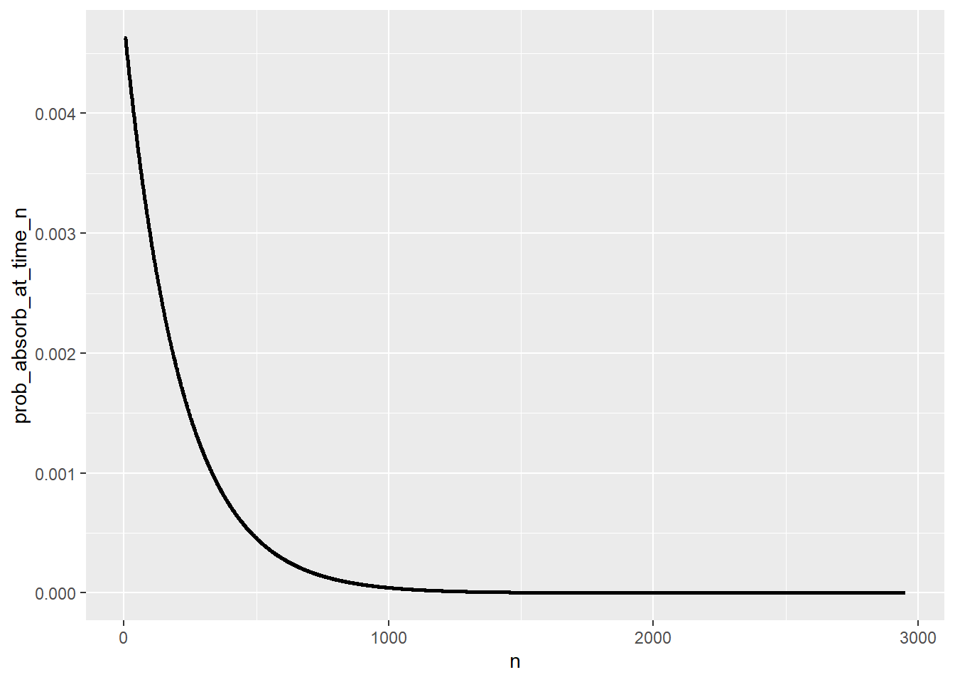
sum(T_pmf[, 1] * T_pmf[, 2])[1] 215.9968Simulation
n_rep = 10000

n_rolls = 3000 # fixed number of rolls instead of while loop

T123 = rep(NA, n_rep)

for (i in 1:n_rep){
  rolls = sample(1:6, n_rolls, replace = TRUE)
  rolls1 = rolls[-c(n_rolls, n_rolls - 1)]
  rolls2 = rolls[-c(1, n_rolls)]
  rolls3 = rolls[-c(1, 2)]
  T123[i] = min(which((rolls1 == 1) &
                        (rolls2 == 2) &
                        (rolls3 == 3))) + 2
}

mean(T123)
[1] 217.5725hist(T123)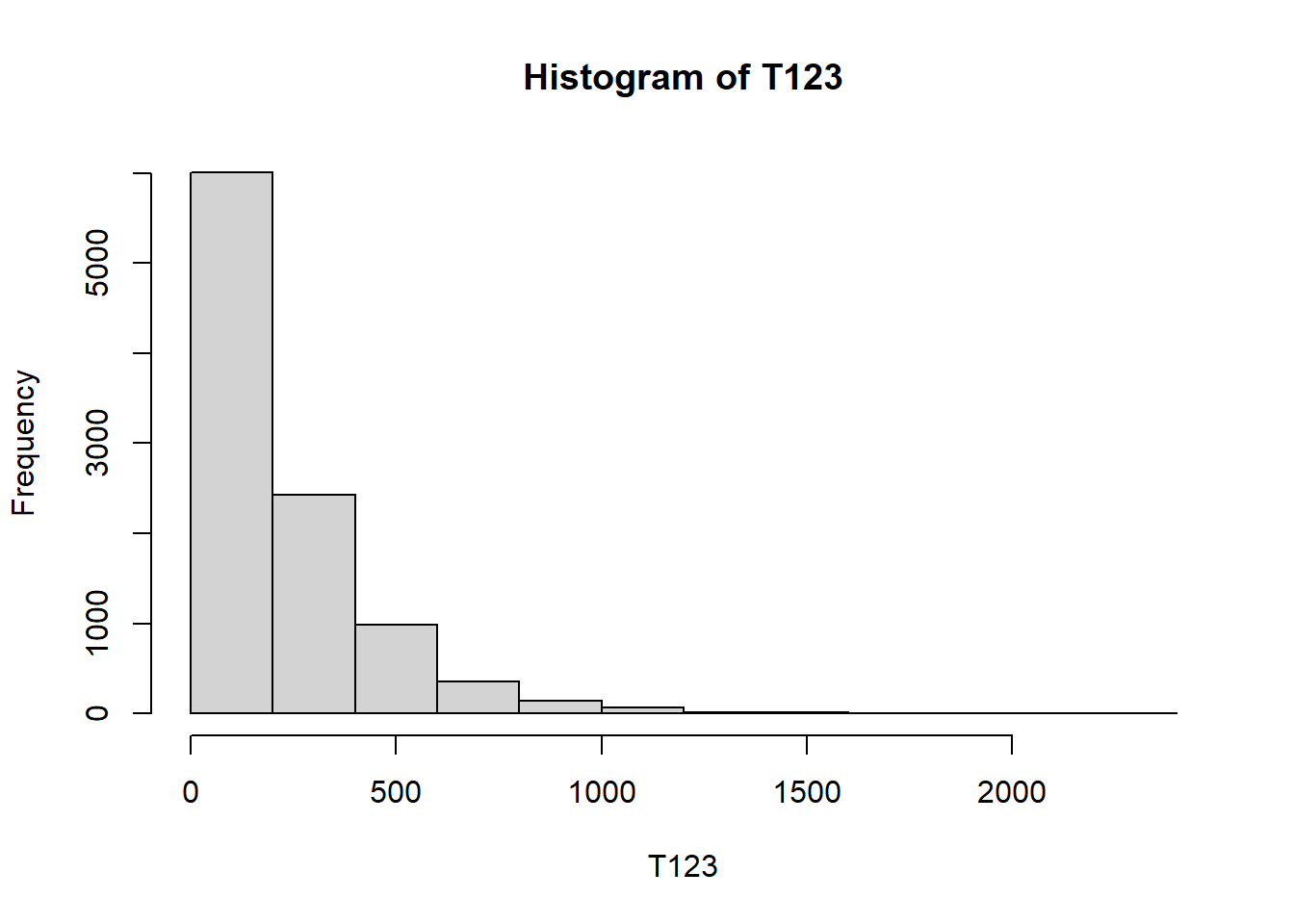
Morty rolls
States: 0 -> 6 -> 66 -> 666
state_names = c("0", "6", "66", "666")

P = rbind(
  c(5, 1, 0, 0),
  c(5, 0, 1, 0),
  c(5, 0, 0, 1),
  c(0, 0, 0, 6)
  ) / 6

mean_time_to_absorption(P, state_names) |>
kbl() |> kable_styling()| start_state | mean_time_to_absorption |
|---|---|
| 0 | 258 |
| 6 | 252 |
| 66 | 216 |
T_pmf = pmf_of_time_to_absorption(P, state_names, start_state = "0")

T_pmf |> head(10) |> kbl() |> kable_styling()| n | prob_absorb_at_time_n |
|---|---|
| 1 | 0.0000000 |
| 2 | 0.0000000 |
| 3 | 0.0046296 |
| 4 | 0.0038580 |
| 5 | 0.0038580 |
| 6 | 0.0038580 |
| 7 | 0.0038402 |
| 8 | 0.0038253 |
| 9 | 0.0038104 |
| 10 | 0.0037955 |
ggplot(T_pmf |>
         filter(prob_absorb_at_time_n > 0),
       aes(x = n,
           y = prob_absorb_at_time_n)) +
  geom_line(linewidth = 1)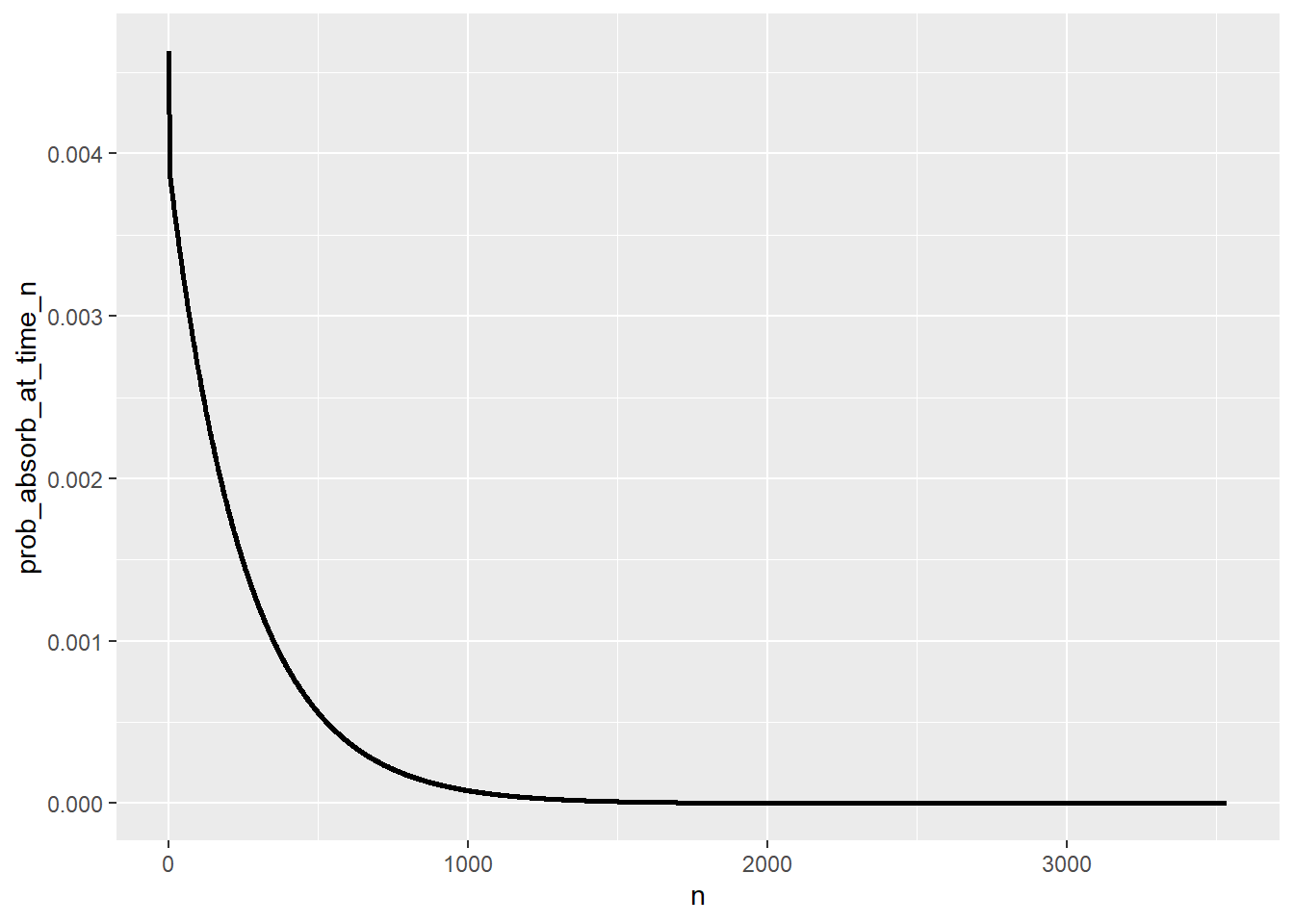
sum(T_pmf[, 1] * T_pmf[, 2])[1] 257.9962Simulation
n_rep = 10000

n_rolls = 3000 # fixed number of rolls instead of while loop

T666 = rep(NA, n_rep)

for (i in 1:n_rep){
  rolls = sample(1:6, n_rolls, replace = TRUE)
  rolls1 = rolls[-c(n_rolls, n_rolls - 1)]
  rolls2 = rolls[-c(1, n_rolls)]
  rolls3 = rolls[-c(1, 2)]
  T666[i] = min(which((rolls1 == 6) &
                        (rolls2 == 6) &
                        (rolls3 == 6))) + 2
}

mean(T666)
[1] 259.6035hist(T666)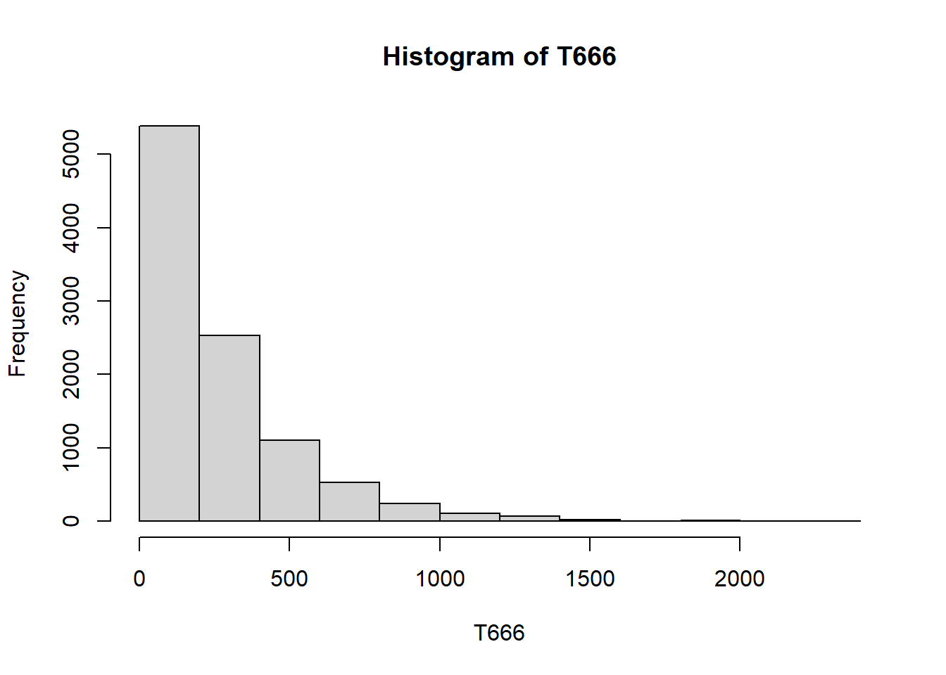
Cube
Q = rbind(
  c(1, 3, 0),
  c(1, 1, 2),
  c(0, 2, 1)
  )/4

solve(diag(3) - Q, rep(1, 3))
[1] 13.333333 12.000000 9.333333Ehrenfest urn chain - absorbing state
M = 5

state_names = 0:M

P = rbind(
  c(5, 0, 0, 0, 0, 0),
  c(1, 0, 4, 0, 0, 0),
  c(0, 2, 0, 3, 0, 0),
  c(0, 0, 3, 0, 2, 0),
  c(0, 0, 0, 4, 0, 1),
  c(0, 0, 0, 0, 0, 5)
) / 5plot_transition_matrix(P, state_names, n_step = 10)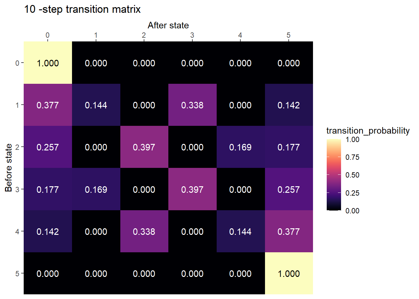
plot_transition_matrix(P, state_names, n_step = 50)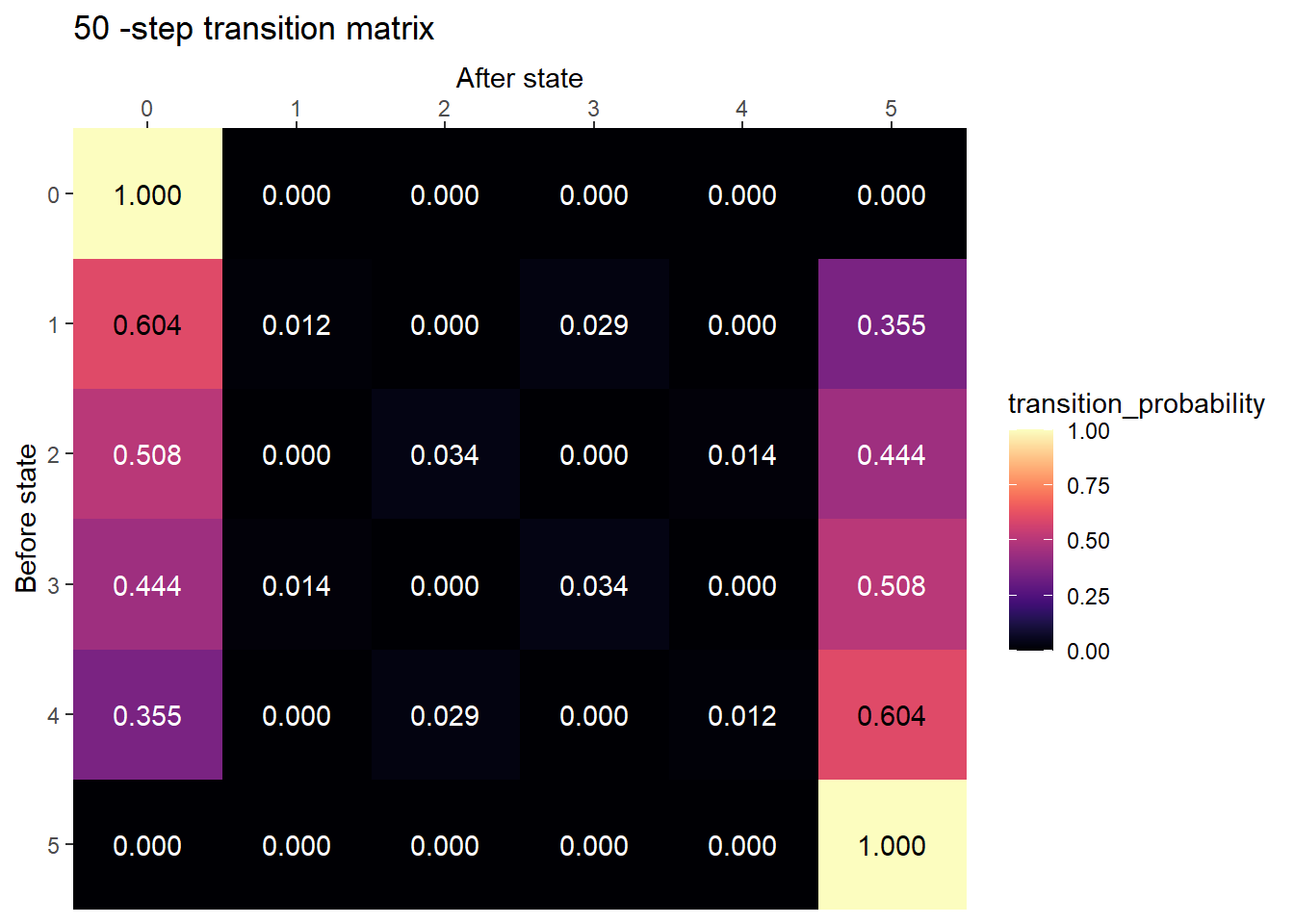
After many steps, the chain is probably absorbed
plot_transition_matrix(P, state_names, n_step = 200)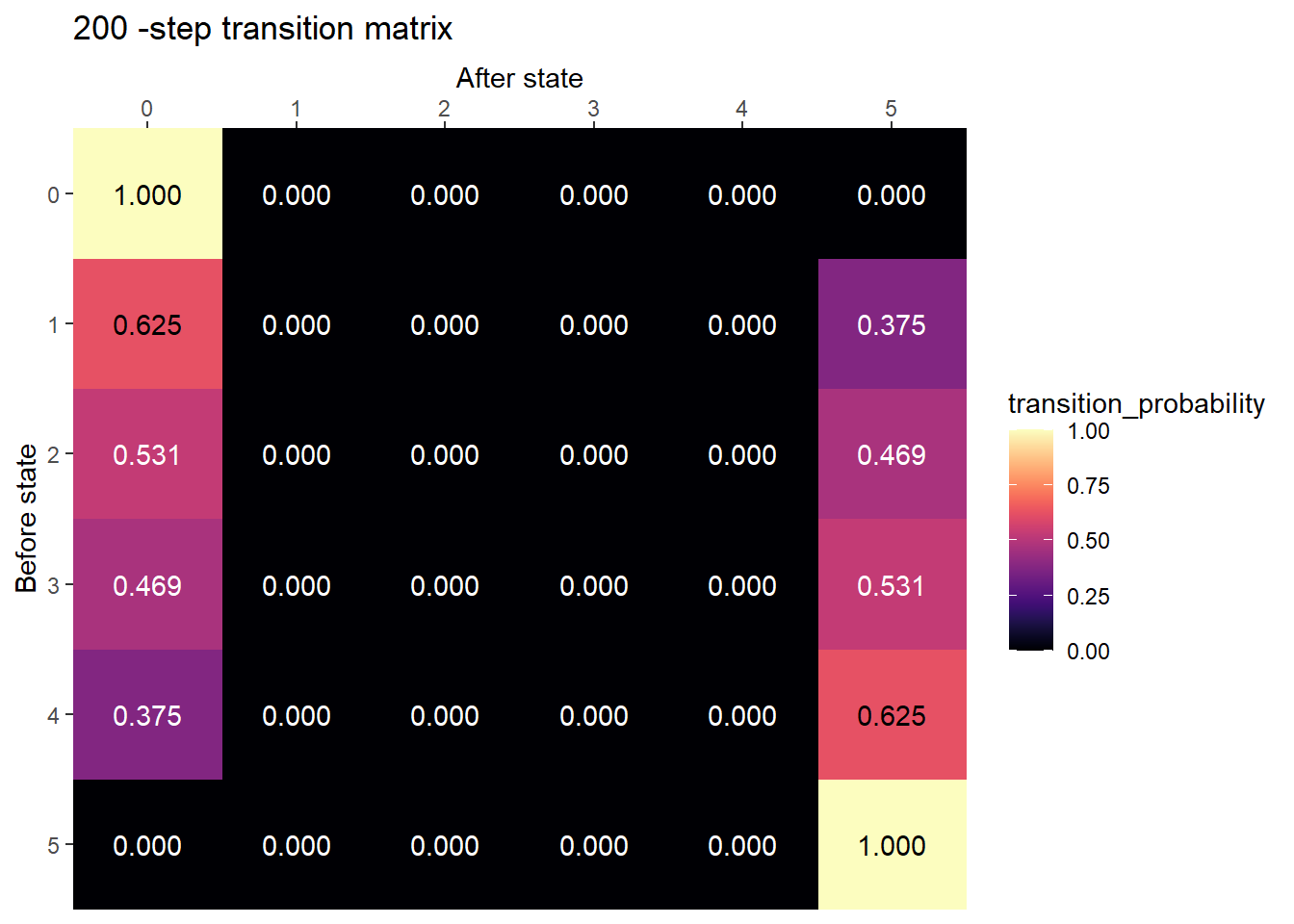
Computing probability of absorption in each state using function
absorption_probability(P, state_names) |>
kbl() |> kable_styling()| start_state | prob_absorb_in_state_0 | prob_absorb_in_state_5 |
|---|---|---|
| 1 | 0.62500 | 0.37500 |
| 2 | 0.53125 | 0.46875 |
| 3 | 0.46875 | 0.53125 |
| 4 | 0.37500 | 0.62500 |
Q = P[2:5, 2:5]
Q
[,1] [,2] [,3] [,4]
[1,] 0.0 0.8 0.0 0.0
[2,] 0.4 0.0 0.6 0.0
[3,] 0.0 0.6 0.0 0.4
[4,] 0.0 0.0 0.8 0.0R = P[2:5, c(1, 6)]
R [,1] [,2]
[1,] 0.2 0.0
[2,] 0.0 0.0
[3,] 0.0 0.0
[4,] 0.0 0.2Pi = solve(diag(4) - Q, R)
Pi [,1] [,2]
[1,] 0.62500 0.37500
[2,] 0.53125 0.46875
[3,] 0.46875 0.53125
[4,] 0.37500 0.62500Rolling until 456 or 666
state_names = c("0", "4", "45", "456", "6", "66", "666")

P = rbind(
  c(4, 1, 0, 0, 1, 0, 0),
  c(3, 1, 1, 0, 1, 0, 0),
  c(4, 1, 0, 1, 0, 0, 0),
  c(0, 0, 0, 6, 0, 0, 0),
  c(4, 1, 0, 0, 0, 1, 0),
  c(4, 1, 0, 0, 0, 0, 1),
  c(0, 0, 0, 0, 0, 0, 6)
) / 6


absorption_probability(P, state_names)
start_state prob_absorb_in_state_456 prob_absorb_in_state_666
1 0 0.5512821 0.4487179
2 4 0.5641026 0.4358974
3 45 0.6282051 0.3717949
4 6 0.5384615 0.4615385
5 66 0.4615385 0.5384615mean_time_to_absorption(P, state_names) start_state mean_time_to_absorption
1 0 119.07692
2 4 115.84615
3 45 99.69231
4 6 116.30769
5 66 99.69231Simulation
n_rep = 10000

n_rolls = 3000 # fixed number of rolls instead of while loop

T_abs = rep(NA, n_rep)
abs_state = rep(NA, n_rep)

for (i in 1:n_rep){
  rolls = sample(1:6, n_rolls, replace = TRUE)
  rolls1 = rolls[-c(n_rolls, n_rolls - 1)]
  rolls2 = rolls[-c(1, n_rolls)]
  rolls3 = rolls[-c(1, 2)]
  T456 = min(which((rolls1 == 4) &
                        (rolls2 == 5) &
                        (rolls3 == 6))) + 2
  T666 = min(which((rolls1 == 6) &
                        (rolls2 == 6) &
                        (rolls3 == 6))) + 2
  T_abs[i] = min(c(T456, T666))
  abs_state[i] = which.min(c(T456, T666))

}

hist(T_abs)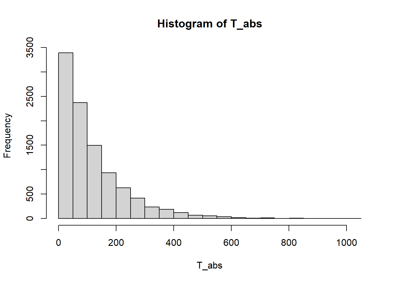
mean(T_abs)[1] 118.1072table(abs_state) / n_repabs_state
1 2
0.5501 0.4499