5 Cleaning & Reshaping
When we talk about cleaning data, there are 4 broad steps:
- Reshaping and tidying
- Filtering and subsetting
- Transforming/re-coding/cleaning variables
- Aggregating and/or merging the data
Steps 2 and 3 we talked about last week, and we will soon talk about step 4.
Step 1 is what we are going to talk about today, and is a topic with a good amount of complexity.
5.1 Unit of Analysis
I have discussed before the importance of knowing the unit of analysis of the data you are working with. This is really going to come into play now.
Once again, to get the unit of analysis ask: what does each row uniquely represent?
Last week when we were working with the ACS data this was very clear as each row represented one of the approximately 3000 counties in the United States.
But this can get more complicated.
Compare this dataset:
#>   county date_1_1_2021 date_1_2_2021 date_1_3_2021
#> 1     c1           990             9           215
#> 2     c2           140          1000           305
#> 3     c3           797           323           141
#> 4     c4           343            34           645
#>   date_1_4_2021
#> 1           646
#> 2             4
#> 3           260
#> 4           785
To this dataset:
#>    county          date covid.cases
#> 1      c1 date_1_1_2021         990
#> 2      c2 date_1_1_2021         140
#> 3      c3 date_1_1_2021         797
#> 4      c4 date_1_1_2021         343
#> 5      c1 date_1_2_2021           9
#> 6      c2 date_1_2_2021        1000
#> 7      c3 date_1_2_2021         323
#> 8      c4 date_1_2_2021          34
#> 9      c1 date_1_3_2021         215
#> 10     c2 date_1_3_2021         305
#> 11     c3 date_1_3_2021         141
#> 12     c4 date_1_3_2021         645
#> 13     c1 date_1_4_2021         646
#> 14     c2 date_1_4_2021           4
#> 15     c3 date_1_4_2021         260
#> 16     c4 date_1_4_2021         785
First notice: these two datasets contain the exact same information. This is data on covid cases in 4 counties for the first 4 days of 2021. The same 16 case numbers exist in both datasets.
What is the unit of analysis of the first dataset, and what is the unit of analysis of the second dataset?
The first dataset has county as the unit of observation. Each row is a county and every county is only in the dataset once.
The second dataset also has county as a variable, but does county uniquely identify each row? No! There are 4 rows for each county, one for each date. In this case the unit of analysis of the data is county-date.
These two datasets, representing the same data, have two different units of analysis.
More broadly, we might consider these two datasets as representing the same data in both “Wide” and “Long” formats.
- Wide data has one observation per row, and columns have data for a particular variable spread out over columns.
- Long data might have observations occur in several rows, but each variable only exists in only one column.
In the above example, the first dataset was wide with respect to county. There is only one row for county, but the data for covid cases was spread across several rows. The second dataset was long with respect to county. Each county existed across multiple rows, but case numbers are represented in only one column.
Here is another example:
#>    district candidate votes
#> 1         1     Biden  1362
#> 2         1     Trump  1073
#> 3         2     Biden  1453
#> 4         2     Trump  1147
#> 5         3     Biden  1481
#> 6         3     Trump  1076
#> 7         4     Biden  1072
#> 8         4     Trump  1495
#> 9         5     Biden  1372
#> 10        5     Trump  1286
What is the unit of analysis of this data? Can it be district? No! there are two rows for every district so district does not uniquely identify rows. What about candidate? No! The candidate also does not uniquely identify rows. Here district-candidate uniquely identifies rows.
And once again, we can represent the same information like this:
#>   district Biden Trump
#> 1        1  1362  1073
#> 2        2  1453  1147
#> 3        3  1481  1076
#> 4        4  1072  1495
#> 5        5  1372  1286
This is the same 10 vote counts now represented in a wide format.
The first dataset is long with respect to district: districts occurred across several rows, but the vote information only existed in one column.
The second dataset is wide with respect to district: districts only exist in one row, but now the vote information is spread across multiple rows.
OK, let’s get even more wild: how would we charecterize this dataset:
#>   candidate    1    2    3    4    5
#> 1     Biden 1362 1453 1481 1072 1372
#> 2     Trump 1073 1147 1076 1495 1286
This is the same information again! Now presented in a new way. Now the unit of analysis is candidate. We would say that this data is wide with respect to candidate. Each candidate is in only one row, and the vote information is spread across multiple columns, one for each district.
Which of these is the “right” way to display this data? There is no such thing! None is right or wrong. The three different versions of this vote data are all helpful for different tasks. Knowing and understanding a particular task requires, and being able to use R to switch between these differently shaped datasets is what is key.
I won’t lie: reshaping is somewhat tricky and I have to look up how to do it pretty much every time I have a task that requires it. But it is also an invaluable step in the data cleaning process.
Let’s jump into how we do reshaping. The tools we are using are also from the tidyr package that we used last week, so we will have to load that in.
First let’s load in the first example from above:
library(tidyr)
dat <- rio::import("https://github.com/marctrussler/IDS-Data/raw/main/WideExample.RDS")
dat
#>   county date_1_1_2021 date_1_2_2021 date_1_3_2021
#> 1     c1           990             9           215
#> 2     c2           140          1000           305
#> 3     c3           797           323           141
#> 4     c4           343            34           645
#>   date_1_4_2021
#> 1           646
#> 2             4
#> 3           260
#> 4           785
We are starting here with wide data that we want to make long. There is one row for each of the 4 counties, and the information for cases is spread across 4 columns.
To go from wide to long data we use the gather() command.
Here are the instructions we need to give gather()
#gather(our dataset,
#       key = what we want to call the new column we are creating that is currently in columns,
#       value = what we want to call the new column that will hold the data currently spread across #columns,
#       which columns contain the data currently)
Applying to this example:
gather(dat,
       key=date,
       value=covid.cases,
       date_1_1_2021:date_1_4_2021)
#>    county          date covid.cases
#> 1      c1 date_1_1_2021         990
#> 2      c2 date_1_1_2021         140
#> 3      c3 date_1_1_2021         797
#> 4      c4 date_1_1_2021         343
#> 5      c1 date_1_2_2021           9
#> 6      c2 date_1_2_2021        1000
#> 7      c3 date_1_2_2021         323
#> 8      c4 date_1_2_2021          34
#> 9      c1 date_1_3_2021         215
#> 10     c2 date_1_3_2021         305
#> 11     c3 date_1_3_2021         141
#> 12     c4 date_1_3_2021         645
#> 13     c1 date_1_4_2021         646
#> 14     c2 date_1_4_2021           4
#> 15     c3 date_1_4_2021         260
#> 16     c4 date_1_4_2021         785
There is nothing special about the names I gave it in this step, I could do:
gather(dat,
       key=batman,
       value=robin,
       date_1_1_2021:date_1_4_2021)
#>    county        batman robin
#> 1      c1 date_1_1_2021   990
#> 2      c2 date_1_1_2021   140
#> 3      c3 date_1_1_2021   797
#> 4      c4 date_1_1_2021   343
#> 5      c1 date_1_2_2021     9
#> 6      c2 date_1_2_2021  1000
#> 7      c3 date_1_2_2021   323
#> 8      c4 date_1_2_2021    34
#> 9      c1 date_1_3_2021   215
#> 10     c2 date_1_3_2021   305
#> 11     c3 date_1_3_2021   141
#> 12     c4 date_1_3_2021   645
#> 13     c1 date_1_4_2021   646
#> 14     c2 date_1_4_2021     4
#> 15     c3 date_1_4_2021   260
#> 16     c4 date_1_4_2021   785
(But I wouldn’t do that).
Like separate() from last week, gather() takes our whole dataset as an argument and outputs a whole dataset. As such, we need to save the output:
#>    county          date covid.cases
#> 1      c1 date_1_1_2021         990
#> 2      c2 date_1_1_2021         140
#> 3      c3 date_1_1_2021         797
#> 4      c4 date_1_1_2021         343
#> 5      c1 date_1_2_2021           9
#> 6      c2 date_1_2_2021        1000
#> 7      c3 date_1_2_2021         323
#> 8      c4 date_1_2_2021          34
#> 9      c1 date_1_3_2021         215
#> 10     c2 date_1_3_2021         305
#> 11     c3 date_1_3_2021         141
#> 12     c4 date_1_3_2021         645
#> 13     c1 date_1_4_2021         646
#> 14     c2 date_1_4_2021           4
#> 15     c3 date_1_4_2021         260
#> 16     c4 date_1_4_2021         785
How do we put this back into its original format?
We can do that with the spread() which takes us from long to wide data. The spread command works like:
#spread(the dataset we are operating on,
#       key = the variable in the dataset we want to make into columns,
#       value = the variable in the dataset we want to put into the key columns)
#
So for this case:
dat.w <- spread(dat.l,
                key=date,
                value=covid.cases)
dat.w
#>   county date_1_1_2021 date_1_2_2021 date_1_3_2021
#> 1     c1           990             9           215
#> 2     c2           140          1000           305
#> 3     c3           797           323           141
#> 4     c4           343            34           645
#>   date_1_4_2021
#> 1           646
#> 2             4
#> 3           260
#> 4           785
For spread, it does matter what the names we put in key and value are, because we are telling R to go get specific columns in the dataset.
What would we do if we wanted a dataset where the unit of analysis is date? Thinking through the spread command, the key variable is the variable we want to make into the columns. If date is the unit of analysis then we have to put county into the columns:
spread(dat.l,
                key=county,
                value=covid.cases)
#>            date  c1   c2  c3  c4
#> 1 date_1_1_2021 990  140 797 343
#> 2 date_1_2_2021   9 1000 323  34
#> 3 date_1_3_2021 215  305 141 645
#> 4 date_1_4_2021 646    4 260 785
Let’s think about the second dataset
dat2
#>    district candidate votes
#> 1         1     Biden  1362
#> 2         1     Trump  1073
#> 3         2     Biden  1453
#> 4         2     Trump  1147
#> 5         3     Biden  1481
#> 6         3     Trump  1076
#> 7         4     Biden  1072
#> 8         4     Trump  1495
#> 9         5     Biden  1372
#> 10        5     Trump  1286
Here this is long data, we have districts spanning across multiple rows, one for each candidate.
We might want this to be wide data if we want a single summation of the election for each district.
Again, to convert from long to wide we need to tell it what column we want in new columns, and where the values are to fill in those cells are:
dat2.w <- spread(dat2,
                 key=candidate,
                 value=votes)

dat2.w
#>   district Biden Trump
#> 1        1  1362  1073
#> 2        2  1453  1147
#> 3        3  1481  1076
#> 4        4  1072  1495
#> 5        5  1372  1286
We went from the unit of analysis being district-candidates, to the unit of analysis being districts.
Then for example, we could calculate each candidates percent of the total vote:
dat2.w$total.votes <- dat2.w$Biden + dat2.w$Trump
dat2.w$perc.biden <- dat2.w$Biden/dat2.w$total.votes
dat2.w$perc.trump <- dat2.w$Trump/dat2.w$total.votes

dat2.w
#>   district Biden Trump total.votes perc.biden perc.trump
#> 1        1  1362  1073        2435  0.5593429  0.4406571
#> 2        2  1453  1147        2600  0.5588462  0.4411538
#> 3        3  1481  1076        2557  0.5791944  0.4208056
#> 4        4  1072  1495        2567  0.4176081  0.5823919
#> 5        5  1372  1286        2658  0.5161776  0.4838224
You don’t often want to delete data, but let’s say we just wanted to make a nice table and only wanted district, perc.biden, perc.trump, and to mak ethe values rounded.
You can delete variables:
dat2.table <- dat2.w
dat2.table$Biden <- NULL
dat2.table$Trump <- NULL
dat2.table$total.votes <- NULL
dat2.table
#>   district perc.biden perc.trump
#> 1        1  0.5593429  0.4406571
#> 2        2  0.5588462  0.4411538
#> 3        3  0.5791944  0.4208056
#> 4        4  0.4176081  0.5823919
#> 5        5  0.5161776  0.4838224
We can also give a list of variables to keep and subset that way:
to.keep <- c("district","perc.biden","perc.trump")
dat2.table <- dat2.w[to.keep]
dat2.w <- dat2.w[to.keep]

dat2.table
#>   district perc.biden perc.trump
#> 1        1  0.5593429  0.4406571
#> 2        2  0.5588462  0.4411538
#> 3        3  0.5791944  0.4208056
#> 4        4  0.4176081  0.5823919
#> 5        5  0.5161776  0.4838224
To round a variable we use…. round()
round(717.128210, 0)
#> [1] 717

dat2.table$perc.biden <- round(dat2.table$perc.biden*100,2)
dat2.table$perc.trump <- round(dat2.table$perc.trump*100,2)

dat2.table
#>   district perc.biden perc.trump
#> 1        1      55.93      44.07
#> 2        2      55.88      44.12
#> 3        3      57.92      42.08
#> 4        4      41.76      58.24
#> 5        5      51.62      48.38
What if we wanted to study candidates, instead of districts?? It should be pretty clear what to do:
dat.2.candidates <- spread(dat2,
                           key=district,
                           value = votes)
dat.2.candidates
#>   candidate    1    2    3    4    5
#> 1     Biden 1362 1453 1481 1072 1372
#> 2     Trump 1073 1147 1076 1495 1286
Again: there is nothing right or wrong about any of these datasets. All of them just present the same information in different ways. Translating in between them
5.2 A Full Data Cleaning Example
In the second half of this week we are going to go through a full example of cleaning a dataset from start to finish.
library(tidyr)
library(lubridate)
#> Warning: package 'lubridate' was built under R version
#> 4.1.3
#>
#> Attaching package: 'lubridate'
#> The following objects are masked from 'package:base':
#>
#>     date, intersect, setdiff, union
Is there a relationship between age and voting for Trump among Millenials? We know that there is definitely a relationship in the population as a whole, but does that same logic extend to within an age group that is very anti Trump?
Could definitely see older millenials maybe being more concerned about taxes?
Today we are going to work with some survey data to ultimately answer that question, but we first have to clean that data to be able to work with it.
5.2.1 Reshaping and reformatting data
Today we’ll be working again Generation Forward survey data.
genfor <- rio::import("https://github.com/marctrussler/IDS-Data/raw/main/Genfor.RDS")The unit of analysis we want to work with are individuals, which in this case are American millenials.
Is it the case that individuals in this dataset are uniquely identified in each row? What other things seem like they need to be cleaned?
head(genfor)
#>     GENF_ID      WEIGHT1 Q0 Q1 approval.party
#> 1 792562474 0.4921835398  2  2     democratic
#> 2 792562474 0.4921835398  2  2     republican
#> 3 794325578 1.2025737846  4  5     democratic
#> 4 794325578 1.2025737846  4  5     republican
#> 5 795569196 0.1318494446  1  5     democratic
#> 6 795569196 0.1318494446  1  5     republican
#>   approval.value Q10A_1 Q10A_2 Q10A_3 Q10A_4 Q10A_5 Q10A_6
#> 1              3      0      0      0      0      0      0
#> 2              2      0      0      0      0      0      0
#> 3              3      0      0      0      0      0      0
#> 4              4      0      0      0      0      0      0
#> 5              2      0      0      0      0      0      0
#> 6              3      0      0      0      0      0      0
#>   Q10A_7 Q10A_8 Q10A_9 Q10A_10 Q10A_11 Q10A_12 Q10A_13
#> 1      0      0      0       0       0       0       0
#> 2      0      0      0       0       0       0       0
#> 3      0      0      0       0       0       0       0
#> 4      0      0      0       0       0       0       0
#> 5      0      0      0       0       0       0       0
#> 6      0      0      0       0       0       0       0
#>   Q10A_14 Q10A_15 Q10A_16 Q10A_17 Q10A_18 Q10A_19 Q10A_20
#> 1       0       0       1       0       0       0       0
#> 2       0       0       1       0       0       0       0
#> 3       0       0       0       0       0       0       0
#> 4       0       0       0       0       0       0       0
#> 5       0       0       0       0       0       0       0
#> 6       0       0       0       0       0       0       0
#>   Q10A_21 Q10A_22 partyid7       date duration     device
#> 1       0       0        5 2017-10-27       11    Desktop
#> 2       0       0        5 2017-10-27       11    Desktop
#> 3       1       0        4 2017-10-27        5 Smartphone
#> 4       1       0        4 2017-10-27        5 Smartphone
#> 5       0       1        3 2017-10-26       11 Smartphone
#> 6       0       1        3 2017-10-26       11 Smartphone
#>   gender age educ state
#> 1      1  18    9    PA
#> 2      1  18    9    PA
#> 3      2  27    6    OK
#> 4      2  27    6    OK
#> 5      2  22   10    NC
#> 6 2 22 10 NC- There are two rows for every observation
- The contents of the Q10A variable are spread across 22 columns
- The column names are inconsistently formatted and not very descriptive
- Most of the variables could be cleaned up a bit so that they’re easier to interpret
Just as a reference for later, I’m going to save an original version of the dataset.
genfor.untouched <- genforJust as a proof of the above, we can compare the number of rows with how many unique entries there are for ID:
Let’s figure this out.
With regard to the approval variable, is the genforward data formatted as wide or long?
head(genfor[c("GENF_ID","approval.party","approval.value")])
#>     GENF_ID approval.party approval.value
#> 1 792562474     democratic              3
#> 2 792562474     republican              2
#> 3 794325578     democratic              3
#> 4 794325578     republican              4
#> 5 795569196     democratic              2
#> 6 795569196     republican              3
Notice that every value of row 1 equals the value in row 2, except for approval.party and approval.value.
genfor[1,] == genfor[2,]
#>   GENF_ID WEIGHT1   Q0   Q1 approval.party approval.value
#> 1    TRUE    TRUE TRUE TRUE          FALSE          FALSE
#>   Q10A_1 Q10A_2 Q10A_3 Q10A_4 Q10A_5 Q10A_6 Q10A_7 Q10A_8
#> 1   TRUE   TRUE   TRUE   TRUE   TRUE   TRUE   TRUE   TRUE
#>   Q10A_9 Q10A_10 Q10A_11 Q10A_12 Q10A_13 Q10A_14 Q10A_15
#> 1   TRUE    TRUE    TRUE    TRUE    TRUE    TRUE    TRUE
#>   Q10A_16 Q10A_17 Q10A_18 Q10A_19 Q10A_20 Q10A_21 Q10A_22
#> 1    TRUE    TRUE    TRUE    TRUE    TRUE    TRUE    TRUE
#>   partyid7 date duration device gender  age educ state
#> 1     TRUE TRUE     TRUE   TRUE   TRUE TRUE TRUE  TRUE
So with respect to the “approval” variables genfor is a long dataset, where each observation (i.e. each survey respondent) has two rows of data. And their approval ratings for the Democratic and Republican parties are split across the two rows.
Our first step in cleaning the data will be to condense those two rows into one.
To do this, we’ll use the spread() function from the tidyr package. We have to tell the function which variable we’ll want to use as our new column names(the “key”) and which variable contains the values that will populate those new columns (the “value”):
genfor <- spread(genfor,
                 key = approval.party,
                 value = approval.value)

head(genfor)
#>     GENF_ID      WEIGHT1 Q0 Q1 Q10A_1 Q10A_2 Q10A_3 Q10A_4
#> 1 792562474 0.4921835398  2  2      0      0      0      0
#> 2 794325578 1.2025737846  4  5      0      0      0      0
#> 3 795569196 0.1318494446  1  5      0      0      0      0
#> 4 803023033 0.8249129727  2  2      1      0      0      0
#> 5 809729125  0.214907857  4  4      0      0      0      0
#> 6 812940493 0.8648717697  1  5      0      0      1      0
#>   Q10A_5 Q10A_6 Q10A_7 Q10A_8 Q10A_9 Q10A_10 Q10A_11
#> 1      0      0      0      0      0       0       0
#> 2      0      0      0      0      0       0       0
#> 3      0      0      0      0      0       0       0
#> 4      0      0      0      0      0       0       0
#> 5      0      0      0      0      0       0       1
#> 6      0      0      0      0      0       0       0
#>   Q10A_12 Q10A_13 Q10A_14 Q10A_15 Q10A_16 Q10A_17 Q10A_18
#> 1       0       0       0       0       1       0       0
#> 2       0       0       0       0       0       0       0
#> 3       0       0       0       0       0       0       0
#> 4       0       0       0       0       0       0       0
#> 5       0       0       0       0       0       0       0
#> 6       0       0       0       0       0       0       0
#>   Q10A_19 Q10A_20 Q10A_21 Q10A_22 partyid7       date
#> 1       0       0       0       0        5 2017-10-27
#> 2       0       0       1       0        4 2017-10-27
#> 3       0       0       0       1        3 2017-10-26
#> 4       0       0       0       0        7 2017-10-29
#> 5       0       0       0       0        2 2017-11-01
#> 6       0       0       0       0        1 2017-10-29
#>   duration     device gender age educ state democratic
#> 1       11    Desktop      1  18    9    PA          3
#> 2        5 Smartphone      2  27    6    OK          3
#> 3       11 Smartphone      2  22   10    NC          2
#> 4        8 Smartphone      1  32   12    TN          4
#> 5       45 Smartphone      2  25   10    NY          1
#> 6        8 Smartphone      2  28   14    NM          2
#>   republican
#> 1          2
#> 2          4
#> 3          3
#> 4          2
#> 5          3
#> 6          4
Notice the other nice thing about the spread function is that it ignored all variables that were the same across the two rows. The only thing that happened is that we got two new variables.
5.2.2 Dealing with individual variables that are spread across multiple columns
Now let’s deal with the Q10A variable. Let’s give it a quick look:
Occasionally (NOT ALWAYS, OR EVEN USUALLY) datsets will come prepackaged with extra information contained within each variable that will tell you some information about the variable and what the values are. We can access that information using the attributes function
attributes(genfor.untouched$Q10A_1)
#> $label
#> [1] "[Abortion] What do you think is the most important problem facing this country?"
#>
#> $format.stata
#> [1] "%8.0g"
#>
#> $labels
#>  No Yes
#>   0   1
attributes(genfor.untouched$Q10A_2)
#> $label
#> [1] "[National debt] What do you think is the most important problem facing this country?"
#>
#> $format.stata
#> [1] "%8.0g"
#>
#> $labels
#>  No Yes
#>   0   1
attributes(genfor.untouched$Q10A_16)
#> $label
#> [1] "[Taxes] What do you think is the most important problem facing this country?"
#>
#> $format.stata
#> [1] "%8.0g"
#>
#> $labels
#>  No Yes
#>   0   1
So it’s the same question, just split across multiple columns, where each column represents a different issue.
(Most of the time this information about variables will be contained in a separate pdf “codebook”.)
So we’re going to want to collapse these 22 columns into one. To do that we’ll use the gather() function, to move these data with respect to this variable into a long format.
We have to tell it the key (which is the new name we want to give our key variable), the value (which is the new name we want to give our values variable), and a vector of all the columns that we’re collapsing/gathering:
genfor <- gather(genfor,
                 key = top.issue, ## we could have called this anything
                 value = val, ## this could be anything also
                 Q10A_1:Q10A_22)
Now let’s see what we have:
nrow(genfor)
#> [1] 41272
#View(genfor)
We went from 1876 rows to tens of thousands
We’ve transferred the unit of observations into individual issue-importance level. For each individual we have a row for how they answered the issue importance question.
We need to get rid of all those extra rows. We’re not actually interested in when a person does not care about an issue. So we can drop all the rowswhere ‘val’ is zero:
genfor <- genfor[genfor$val != 0,]
nrow(genfor)
#> [1] 2149
That got us most of the way there, but we’ve still got more rows than we should? What’s going on?
#View(genfor)All the people who didn’t answer the question were coded as 99 for every issue. So now there’s 22 rows for each of those people.
What we want is one row per person. We’ll use the duplicated() function to do this. This function takes a vector and returns a FALSE if it’s the first time this value has shown up in the vector, and a TRUE if it’s appeared before.
head(duplicated(genfor$GENF_ID))
#> [1] FALSE FALSE FALSE FALSE FALSE FALSE
If we use the ! to flip the TRUEs and FALSEs, then we’ll have a vector we can useto ensure that we only have one row per person:
genfor <- genfor[!duplicated(genfor$GENF_ID),]
head(genfor)
#>        GENF_ID      WEIGHT1 Q0 Q1 partyid7       date
#> 4    803023033 0.8249129727  2  2        7 2017-10-29
#> 9    831421601 1.3049241841  2  1        7 2017-10-26
#> 107 1219666547 0.1913640053  3  2        2 2017-10-26
#> 149 1364524431 3.8634938329  2  1        7 2017-10-27
#> 180 1465399167  1.263106426 98 98       -1 2017-11-01
#> 182 1476757020 1.1191845832  3  3        7 2017-10-26
#>     duration     device gender age educ state democratic
#> 4          8 Smartphone      1  32   12    TN          4
#> 9         12    Desktop      2  23   10    CA          4
#> 107        9 Smartphone      1  26   11    IL          2
#> 149        8 Smartphone      2  32    9    UT          4
#> 180     8965 Smartphone      2  25    9    GA         NA
#> 182       10 Smartphone      2  19    9    WA          4
#>     republican top.issue val
#> 4            2    Q10A_1   1
#> 9            1    Q10A_1   1
#> 107          4    Q10A_1   1
#> 149          1    Q10A_1   1
#> 180         NA    Q10A_1  99
#> 182          2    Q10A_1   1
Now we have one last step. We don’t need to keep both ‘top.issue’ and ‘val’. ‘top.issue’ gives us all the information we need, except for the people whowere 99’s in ‘val’. So let’s set ‘top.issue’ to NA for those people, and then we can drop the ‘val’ variable.
genfor$top.issue[genfor$val == 99] <- NA
genfor$val <- NULL
5.2.3 Cleaning column names
What are some of the issues with our column names?
names(genfor)
#>  [1] "GENF_ID"    "WEIGHT1"    "Q0"         "Q1"
#>  [5] "partyid7"   "date"       "duration"   "device"
#>  [9] "gender"     "age"        "educ"       "state"
#> [13] "democratic" "republican" "top.issue"
Remember that the column names are simply stored as a character vector in one of the attributes of a dataframe.
We can manipulate this attribute just like any other attribute of an object.Let’s use the tolower() function to convert all the column names to lowercase:
Now let’s give some of the other variables more descriptive names.
names(genfor)
#>  [1] "genf_id"    "weight1"    "q0"         "q1"
#>  [5] "partyid7"   "date"       "duration"   "device"
#>  [9] "gender"     "age"        "educ"       "state"
#> [13] "democratic" "republican" "top.issue"
attributes(genfor.untouched$Q0) # this one is 2016 presidential vote
#> $label
#> [1] "Did you vote for Hillary Clinton, Donald Trump, someone else, or not vote in the 2016 presidential election?"
#>
#> $format.stata
#> [1] "%8.0g"
#>
#> $labels
#>                                Hillary Clinton
#>                                              1
#>                                   Donald Trump
#>                                              2
#>                                   Someone else
#>                                              3
#> Did not vote in the 2016 presidential election
#>                                              4
#>                                 SKIPPED ON WEB
#>                                             98
#>                                        refused
#>                                             99
attributes(genfor.untouched$Q1) # this one is Trump approval
#> $label
#> [1] "Overall, do you approve, disapprove or neither approve nor disapprove of the way that President Donald Trump is doing his job?"
#>
#> $format.stata
#> [1] "%8.0g"
#>
#> $labels
#>               Strongly approve
#>                              1
#>               Somewhat approve
#>                              2
#> Neither approve nor disapprove
#>                              3
#>            Somewhat disapprove
#>                              4
#>            Strongly disapprove
#>                              5
#>                 SKIPPED ON WEB
#>                             98
#>                        refused
#>                             99
We can, if we like, rename things in this way. Accessing the particular entry in the names vector and assigning a new value
names(genfor)[3] <- "vote2016"A slightly quicker solution is to use the rename() function from dplyr. We have to specify the dataframe we’re manipulating, then tell the function the old and new names of the columns in the format: ‘newname = oldname’. We don’t need to use any quotation marks with this function.
#install.packages("dplyr")
genfor <- dplyr::rename(genfor,
                 weight = weight1,
                 approve.trump = q1,
                 approve.dem = democratic,
                 approve.rep = republican)
head(genfor)
#>        genf_id       weight vote2016 approve.trump partyid7
#> 4    803023033 0.8249129727        2             2        7
#> 9    831421601 1.3049241841        2             1        7
#> 107 1219666547 0.1913640053        3             2        2
#> 149 1364524431 3.8634938329        2             1        7
#> 180 1465399167  1.263106426       98            98       -1
#> 182 1476757020 1.1191845832        3             3        7
#>           date duration     device gender age educ state
#> 4   2017-10-29        8 Smartphone      1  32   12    TN
#> 9   2017-10-26       12    Desktop      2  23   10    CA
#> 107 2017-10-26        9 Smartphone      1  26   11    IL
#> 149 2017-10-27        8 Smartphone      2  32    9    UT
#> 180 2017-11-01     8965 Smartphone      2  25    9    GA
#> 182 2017-10-26       10 Smartphone      2  19    9    WA
#>     approve.dem approve.rep top.issue
#> 4             4           2    Q10A_1
#> 9             4           1    Q10A_1
#> 107           2           4    Q10A_1
#> 149           4           1    Q10A_1
#> 180          NA          NA      <NA>
#> 182           4           2    Q10A_1
names(genfor)
#>  [1] "genf_id"       "weight"        "vote2016"
#>  [4] "approve.trump" "partyid7"      "date"
#>  [7] "duration"      "device"        "gender"
#> [10] "age"           "educ"          "state"
#> [13] "approve.dem"   "approve.rep"   "top.issue"
I’ve got a personal pet-peeve about having underscores in column names. Let’s substitute the underscore in ‘genf_id’ for a period.
We’ll use gsub() to substitute the _ for a .
5.2.4 Recoding values in a vector or in the column of a dataframe
The first thing we want to do is make sure our variables are the correct type of data (i.e. character, numeric, logical, etc)
summary(genfor)
#>     genf.id                   weight        vote2016
#>  Min.   :7.926e+08   0.229665156 :  14   Min.   : 1.000
#>  1st Qu.:2.571e+09   0.2958000119:  14   1st Qu.: 1.000
#>  Median :4.293e+09   0.255285515 :  12   Median : 2.000
#>  Mean   :4.303e+09   0.305879976 :  12   Mean   : 2.576
#>  3rd Qu.:6.048e+09   0.1508269493:   9   3rd Qu.: 4.000
#>  Max.   :7.875e+09   0.39396181  :   9   Max.   :99.000
#>                      (Other)     :1806
#>  approve.trump       partyid7          date
#>  Min.   : 1.000   Min.   :-1.000   Length:1876
#>  1st Qu.: 3.000   1st Qu.: 2.000   Class :character
#>  Median : 5.000   Median : 3.000   Mode  :character
#>  Mean   : 4.721   Mean   : 3.121
#>  3rd Qu.: 5.000   3rd Qu.: 4.000
#>  Max.   :99.000   Max.   : 7.000
#>
#>     duration        device              gender
#>  Min.   :    1   Length:1876        Min.   :1.000
#>  1st Qu.:    9   Class :character   1st Qu.:1.000
#>  Median :   14   Mode  :character   Median :2.000
#>  Mean   : 1184                      Mean   :1.531
#>  3rd Qu.:   82                      3rd Qu.:2.000
#>  Max.   :19341                      Max.   :2.000
#>  NA's   :2
#>       age             educ          state
#>  Min.   :18.00   Min.   : 1.00   Length:1876
#>  1st Qu.:21.00   1st Qu.: 9.00   Class :character
#>  Median :25.00   Median :10.00   Mode  :character
#>  Mean   :25.15   Mean   :10.28
#>  3rd Qu.:29.00   3rd Qu.:12.00
#>  Max.   :34.00   Max.   :14.00
#>
#>   approve.dem     approve.rep     top.issue
#>  Min.   :1.000   Min.   :1.000   Length:1876
#>  1st Qu.:2.000   1st Qu.:3.000   Class :character
#>  Median :2.000   Median :4.000   Mode  :character
#>  Mean   :2.414   Mean   :3.241
#>  3rd Qu.:3.000   3rd Qu.:4.000
#>  Max.   :4.000   Max.   :4.000
#>  NA's   :242     NA's   :277

class(genfor$weight)
#> [1] "factor"
There’s something wrong with the ‘weight’ variable. It should be numeric, but it doesn’t have summary stats presented about it like the other numeric variables.
is.numeric(genfor$weight)
#> [1] FALSE

is.factor(genfor$weight)
#> [1] TRUE
So the weight variable, which should be numeric, is being stored as a factor. A factor variable is a special type of variable that contains both numeric and descriptive information. To be honest: they are a bit of a holdover from older stats programs like STATA and SPSS. They will have some important funcitonality in regression, but for right now we need to change that so that we can properly use the weights.
The obvious (but annoyingly wrong) way to do this would simply be to use the as.numeric() function to change the weights into numbers. But if you apply as.numeric() to a factor variable, it converts all the values to their arbitrary numeric values rather than their meaningful labels.
head(as.numeric(genfor$weight)) # wrong
#> [1]  992 1206  264 1540 1191 1132
We can get around this problem by first converting the weights into characters and then converting the character strings into numeric
head(as.numeric(as.character(genfor$weight)))
#> [1] 0.824913 1.304924 0.191364 3.863494 1.263106 1.119185
I can’t tell you how frustratingly common this issue is, which is why I’m point it out now. You’re most likely to encounter it when you read in a datasetfrom a spreadsheet, and R turns some of your columns into factors rather than numeric.
We can confirm that this was the right choice by looking at a summary of the two attempts:
summary(as.numeric(genfor$weight))
#>    Min. 1st Qu.  Median    Mean 3rd Qu.    Max.
#>     1.0   366.8   716.5   765.1  1162.2  1627.0
summary(as.numeric(as.character(genfor$weight)))
#>     Min.  1st Qu.   Median     Mean  3rd Qu.     Max.
#>  0.01762  0.24216  0.47743  1.00000  1.18315 10.69962
So now let’s store the corrected weights in the dataset:
genfor$weight <- as.numeric(as.character(genfor$weight))Let’s fix the date:
head(genfor$date)
#> [1] "2017-10-29" "2017-10-26" "2017-10-26" "2017-10-27"
#> [5] "2017-11-01" "2017-10-26"
class(genfor$date)
#> [1] "character"

genfor$date <- ymd(genfor$date)
class(genfor$date)
#> [1] "Date"
This is particularly useful if you’re interested in subsetting the data based on the dates. Let’s say I just want to look at the people who completed in November:
table(genfor$date)
#>
#> 2017-10-26 2017-10-27 2017-10-28 2017-10-29 2017-10-30
#>        542        390        107        246        229
#> 2017-10-31 2017-11-01 2017-11-02 2017-11-03 2017-11-04
#>        103        100         44         41         12
#> 2017-11-05 2017-11-06 2017-11-07 2017-11-08 2017-11-09
#>         18         10         15          7         11
#> 2017-11-10
#>          1

#View(genfor[genfor$date >= "2017-11-01",])
5.2.5 Recoding and replacing values
The most common form of data cleaning is recoding variables. There are tons of different ways to do this in R.
The most basic is recoding by taking advantage of the bracket notation.
Let’s work on recoding the vote2016 (formerly Q0) variable, which is a question about 2016 presidential vote
table(genfor$vote2016)
#>
#>   1   2   3   4  98  99
#> 896 262 213 497   6   2
attributes(genfor.untouched$Q0)
#> $label
#> [1] "Did you vote for Hillary Clinton, Donald Trump, someone else, or not vote in the 2016 presidential election?"
#>
#> $format.stata
#> [1] "%8.0g"
#>
#> $labels
#>                                Hillary Clinton
#>                                              1
#>                                   Donald Trump
#>                                              2
#>                                   Someone else
#>                                              3
#> Did not vote in the 2016 presidential election
#>                                              4
#>                                 SKIPPED ON WEB
#>                                             98
#>                                        refused
#>                                             99
So let’s set the 98 and 99 responses to missing
genfor$vote2016[genfor$vote2016 %in% c(98,99)] <- NA
summary(genfor$vote2016)
#>    Min. 1st Qu.  Median    Mean 3rd Qu.    Max.    NA's
#>   1.000   1.000   2.000   2.166   4.000   4.000       8
table(genfor$vote2016)
#>
#>   1   2   3   4
#> 896 262 213 497
Similarly can use characters to recode
genfor$vote2016[genfor$vote2016==1] <- "Clinton"
genfor$vote2016[genfor$vote2016==2] <- "Trump"
genfor$vote2016[genfor$vote2016==3] <- "Other"
genfor$vote2016[genfor$vote2016 %in% c(4,98,99)] <- NA
table(genfor$vote2016)
#>
#> Clinton   Other   Trump
#>     896     213     262
head(genfor$vote2016)
#> [1] "Trump" "Trump" "Other" "Trump" NA      "Other"
Clean data often has labels that are more descriptive than just arbitrary numbers. So we might recode the gender variable:
attributes(genfor.untouched$gender)
#> $label
#> [1] "Respondent gender"
#>
#> $format.stata
#> [1] "%8.0g"
#>
#> $labels
#> Unknown    Male  Female
#>       0       1       2

genfor$gender[genfor$gender == 1] <- "M"
genfor$gender[genfor$gender == 2] <- "F"
genfor$gender[genfor$gender == 0] <- "U"
My personal preference, however, is to have indicator variables for categories like this.
genfor$female <- NA
genfor$female[genfor$gender=="M" | genfor$gender=="U"] <- 0
genfor$female[genfor$gender=="F"] <- 1
his displays the same information, but in a way that we can do math on, which is helpful.
One last function… If a column contains information about more than one variable we might want to divide it into two columns using the separate() function.
Let’s imagine we wanted separate columns for year, month, and day that the respondent took the survey:
genfor2 <- separate(genfor,
         col = "date",
         into = c("year","month","day"))
head(genfor2)
#>        genf.id   weight vote2016 approve.trump partyid7
#> 4    803023033 0.824913    Trump             2        7
#> 9    831421601 1.304924    Trump             1        7
#> 107 1219666547 0.191364    Other             2        2
#> 149 1364524431 3.863494    Trump             1        7
#> 180 1465399167 1.263106     <NA>            98       -1
#> 182 1476757020 1.119185    Other             3        7
#>     year month day duration     device gender age educ
#> 4   2017    10  29        8 Smartphone      M  32   12
#> 9   2017    10  26       12    Desktop      F  23   10
#> 107 2017    10  26        9 Smartphone      M  26   11
#> 149 2017    10  27        8 Smartphone      F  32    9
#> 180 2017    11  01     8965 Smartphone      F  25    9
#> 182 2017    10  26       10 Smartphone      F  19    9
#>     state approve.dem approve.rep top.issue female
#> 4      TN           4           2    Q10A_1      0
#> 9      CA           4           1    Q10A_1      1
#> 107    IL           2           4    Q10A_1      0
#> 149    UT           4           1    Q10A_1      1
#> 180    GA          NA          NA      <NA>      1
#> 182    WA           4           2    Q10A_1      1
The function will attempt to automatically detect and guess the character that separates the columns. In this case it works just fine, but it’s not a bad idea to specify exactly what you want, so that it doesn’t make an unexpected mistake:
5.2.6 Analysis
Let’s look at doing a quick analysis. Let’s see how age relates to voting for Trump
Let’s first make a variable that is vote for trump (1) or not (0)
genfor$trump <- NA
genfor$trump[genfor$vote2016=="Trump"]<- 1
genfor$trump[genfor$vote2016!="Trump"]<- 0

table(genfor$trump)
#>
#>    0    1
#> 1109  262
(remember this is a survey of millenials, so very few voting for trump)
How does age relate to voting for trump?
making a scatterplot not very helpful here:
plot(genfor$age,genfor$trump)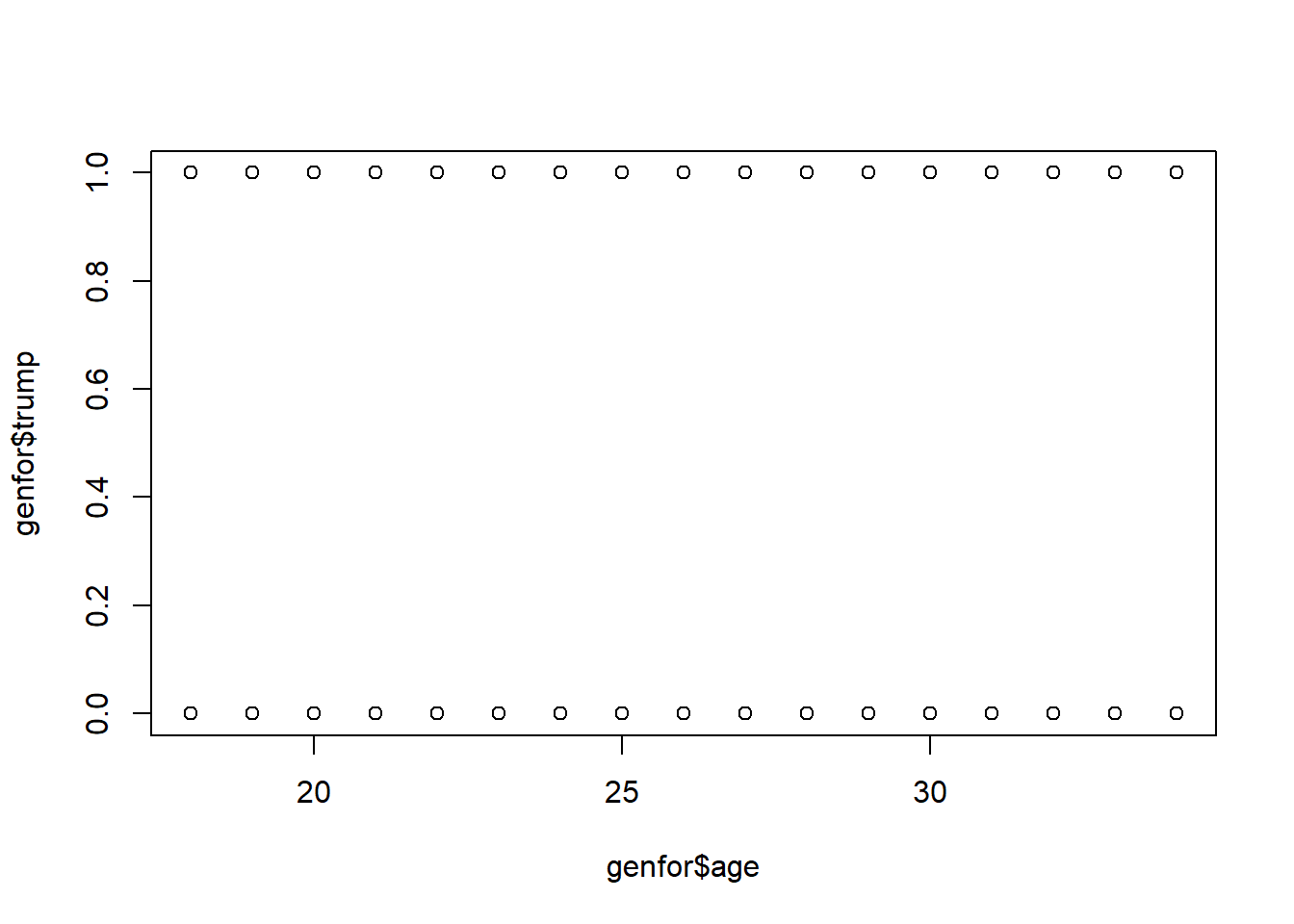
Another possibility is a boxplot where we look at the distribution of ages for trump and not trump voters
boxplot(genfor$age ~ genfor$trump,
        xlab="Vote for Trump",
        ylab="Age",
        main="Distribution of Age for Trump and Non-Trump Voters")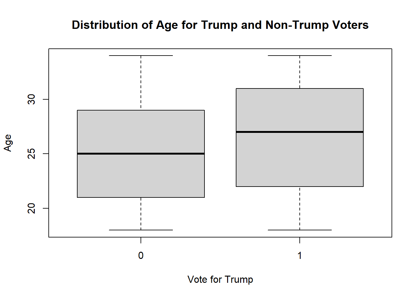
Can also look at the correlation
cor(genfor$age, genfor$trump)
#> [1] NA
cor(genfor$age, genfor$trump, use="pairwise.complete")
#> [1] 0.1280754
Small positive correlation
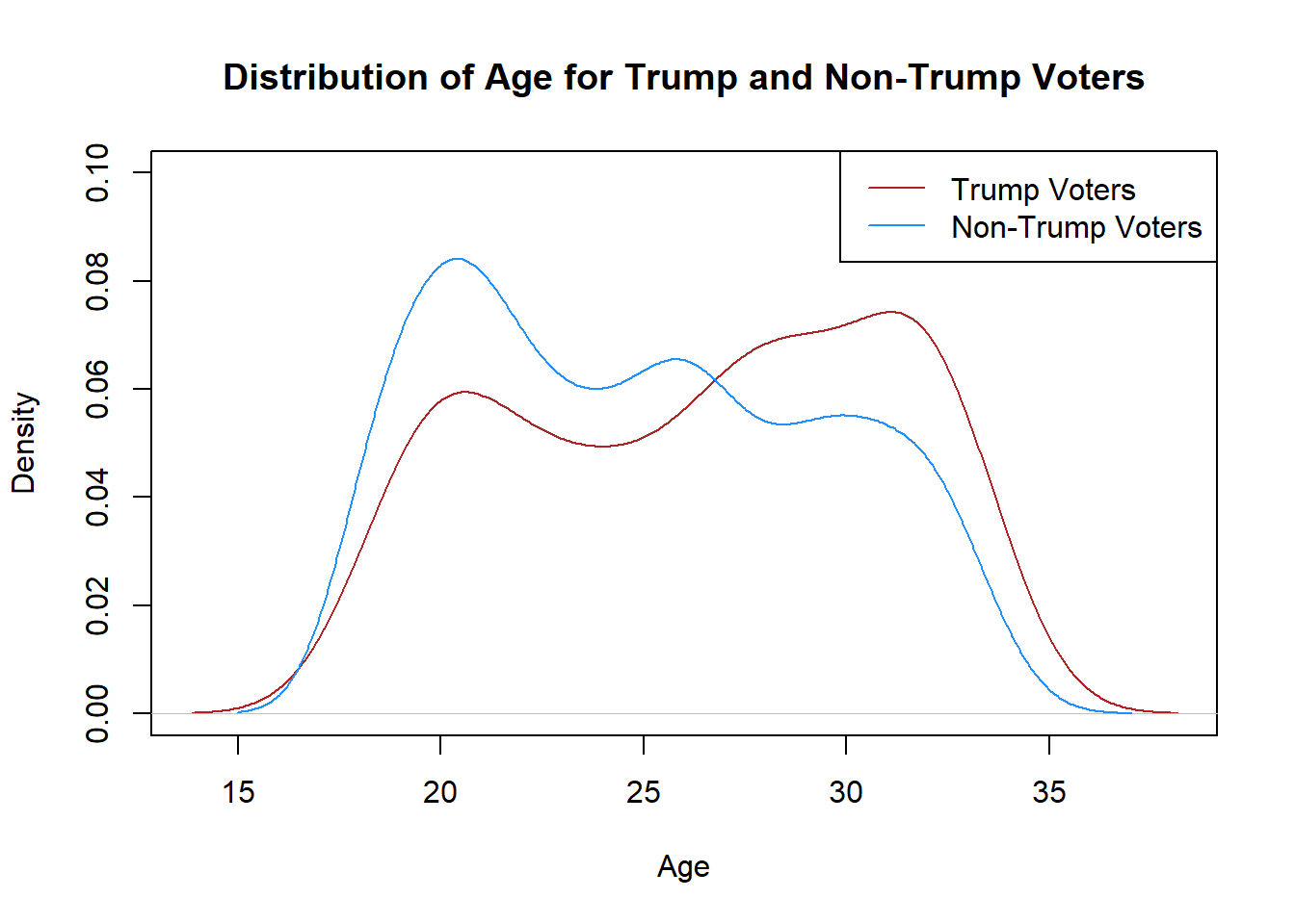
Another way to look at the distribution of age is a density plot
plot(density(genfor$age[genfor$trump==1],na.rm=T),
     xlab="Age",
     main="Distribution of Age for Trump and Non-Trump Voters",
     col="firebrick",
     ylim=c(0,0.1))
points(density(genfor$age[genfor$trump==0],na.rm=T), type="l",
       col="dodgerblue")
legend("topright",c("Trump Voters","Non-Trump Voters"),
       lty=c(1,1), col=c("firebrick","dodgerblue"))