1 What is Data?
To produce good work in data science you need three interlocking sets of skills:
- Domain knowledge in the area you are working;
- Computational knowledge to literally process inputs and produce outputs.
- Statistical knowledge to guide decisions and to interpret findings.
My work at NBC is a good example of how these three things come together. I (and our team more broadly!) have the technical ability to write code that takes raw election returns and produces models. The models I choose and the way that I interpret them are guided by my years of experience in political science. My ability to form conclusions based on the data I am seeing is based on my knowledge of mathematical statistics. All three of these things have to work in concert for me to be a good analyst.
This course is primarily going to focus on (2). And there is a lot to focus on there! Learning how to use R to load, merge and clean data is hard! As is using R to generate output and figures. That is definitely a course-worth of material.
But it’s important to remember that this is only one leg of a three-legged stool.
Domain knowledge you are going to get in your other classes and through your life experience. Whether it’s politics, business, sports, economics… Over time you will gain knowledge of theories that guide behavior in those fields, learn what is important to people etc.
Statistics knowledge will take a specific investment from you to improve. And I highly recommend you make that investment. Even if you have already taken AP stats, it is incredibly helpful to re-learn the basics of statistics at the college level. (Seriously, it is hard to spend too much time on the basics).
The purpose of today’s lesson is to give you an intuitive and non-mathematical introduction to what “statistics” is. This is something for you to keep in mind as we spend time building your technical skills in this class.
1.1 Why isn’t this class “statistics”?
In this class we are going to be working with data, making tables and figures, generating values like the mean, or median… by all normal definitions this is “statistics”. But it’s not, really.
Let’s think about three questions we may want to ask in a political science context. All of these questions pertain to looking back at 2020 and thinking about the inter-relationships of COVID and partisanship:
- Did the majority of Americans approve of how President Trump handled COVID?
- Did Democrats socially distance more than Republicans?
- Did an increase in the number of COVID cases in a person’s area make it more likely that they will socially distance?
What is critical to understand about each of these questions is that none of them are about what is happening in a dataset. They are more general than that. We are interested in what is going on in the real world, not simply in describing what is happening inside some data.
Let’s say we are most interested in the second question in this sequence: “Did Democrats socially distance more than Republicans?”. I might find a survey of 100 Americans from that time period and, among those that took the survey, 5% of Democrats reported going to a restaurant in the previous 24 hours while 9% of Republicans reported doing so.
In this case, there is clearly an association between political party and social distancing for these 100 people.
But my question was not “Do the Democrats in this sample socially distance more than Republicans in this sample?”, my question was about the truth for all of the Democrats and Republicans in America.
Am I any closer to answering that question? What can I say about the truth? Maybe this is a super weird sample of Americans and the truth is that there is no relationship, or that Republicans were the ones that socially distanced more.
Here’s a more fundamental question to think about: If we had surveyed another randomly selected group of people would we have gotten exactly the same answer? Clearly not. But how different would the two samples be?
These questions get us to what is more fundamental about statistics.
1.2 So, what is data?
What might this look like? Let’s take a look at what a dataset that describes this relationship between partisanship and going to a restaurant in the last 7 days might look like:
## Note that I am leaving all of the code in this file so that you have it for your records, though I don't expect you to know
# how any of this works at this point.
# You may want to return to this code at the end of the course to see what you understand!
# A lot of the things I am doing in this lecture form the basis of PSCI1801.

#Generate dataset
set.seed(19144)
democrat <- sample(c(T,F),100, replace=T)
restaurant.prob <- runif(100,0,1) - democrat*.05
restaurant <- NA
restaurant[restaurant.prob>=.5] <- T
restaurant[restaurant.prob<.5] <- F
data <- cbind.data.frame(democrat,restaurant)
head(data,10)
#>    democrat restaurant
#> 1      TRUE      FALSE
#> 2     FALSE      FALSE
#> 3      TRUE       TRUE
#> 4      TRUE       TRUE
#> 5     FALSE       TRUE
#> 6      TRUE      FALSE
#> 7      TRUE      FALSE
#> 8     FALSE      FALSE
#> 9     FALSE       TRUE
#> 10     TRUE       TRUE
Above are the first 10 rows of a dataset describing how individuals break down on partisanship and restaurant attendance. Each row in a dataset represents one of the units we are analyzing. In this case a row is a person. The columns represent attributes of each individual. The first column tells us whether a person is a democrat, or not. In this case this variable can be either true or false. The second column tells us whether that same person has been to a restaurant, or not. So the first person in the dataset is not a democrat and has not been to a restaurant. The second person is a democrat and has been to a restaurant, and so on.
First, what proportion of people have been to a restaurant?
mean(data$restaurant)
#> [1] 0.49
I am using proportions here, which range from 0 to 1. We can transform proportions to percentages by multiplying by 100. So 49% of people in this sample have been to a restaurant.
We want to look at how this number is different for Republicans and Democrats. In a few weeks you will be able to see exactly how this code works. For right now you can just believe me that this is right:
restaurant.dem <- mean(data$restaurant[data$democrat==T])
restaurant.rep <- mean(data$restaurant[data$democrat==F])

restaurant.dem
#> [1] 0.45
restaurant.rep
#> [1] 0.55

restaurant.dem - restaurant.rep
#> [1] -0.1
We see here that around 45% of Democrats have been to a restaurant while 55% of Republicans have. A difference of 10%.
OK, so that is some data and some basic analysis of the data. What is the problem here?
Again: our goal is not to simply describe this dataset….
What would happen if we got a second sample of 100 people. Are we going to get exactly the same result? A difference of 4%? Of course not. Here is a second sample:
set.seed(197)
democrat <- sample(c(T,F),100, replace=T)
restaurant.prob <- runif(100,0,1) - democrat*.05
restaurant <- NA
restaurant[restaurant.prob>=.5] <- T
restaurant[restaurant.prob<.5] <- F
data <- cbind.data.frame(democrat,restaurant)
head(data,10)
#>    democrat restaurant
#> 1      TRUE      FALSE
#> 2      TRUE      FALSE
#> 3      TRUE      FALSE
#> 4     FALSE      FALSE
#> 5     FALSE      FALSE
#> 6      TRUE       TRUE
#> 7      TRUE       TRUE
#> 8      TRUE      FALSE
#> 9     FALSE      FALSE
#> 10     TRUE      FALSE
restaurant.dem <- mean(data$restaurant[data$democrat==T])
restaurant.rep <- mean(data$restaurant[data$democrat==F])

restaurant.dem
#> [1] 0.4716981
restaurant.rep
#> [1] 0.4042553

restaurant.dem - restaurant.rep
#> [1] 0.06744279
Indeed, this second sample gives us a dramatically different result. The Republicans in this sample were actually less likely to go to restaurants than the Democrats. This is a sample from the same population yet it gave us a very different result.
Here are 6 more samples, and in each I’ll calculate the difference between the Democratic proportion going to restaurants and the Republican proportion going to restaurants.
dem.diff <- NA

for(i in 1:6){
democrat <- sample(c(T,F),100, replace=T)
restaurant.prob <- runif(100,0,1) - democrat*.05
restaurant <- NA
restaurant[restaurant.prob>=.5] <- T
restaurant[restaurant.prob<.5] <- F
data <- cbind.data.frame(democrat,restaurant)
dem.diff[i] <- mean(data$restaurant[data$democrat==T]) - mean(data$restaurant[data$democrat==F])
}
dem.diff
#> [1] -0.06000000 -0.05299077  0.03693296  0.08173077
#> [5] -0.04807692  0.06000000
Across these 6 samples of 100 people we had scenarios as different as Republicans being 6 percentage-points more likely to go to restaurants to Democrats being 8 percentage points more likely.
There are, in fact, an infinite number of possible datasets here, which means there are an infinite number of possible differences in these two proportions.
Let me ask this question, which I just want you to think about qualitatively: given those six values, are you confident that the true difference between the amount Democrats and Republicans go to restaurants is not 0? In other words, given what we have seen in terms of the inherent noise of this data being generated, are we confident that we can discern a signal?
I’m not! Given how frequently we get samples where Republicans go to restaurants more often. In general it’s just jumping around so much I’m not confident we are going to be able to pull anything meaningful from this.
“Statistics” is the science of saying: given the noise inherent in our estimates (here the difference in how frequently Democrats and Republicans go to restaurants) what can I conclude about the truth?
1.3 Coin Flip Modelling
We can examine this type of thinking with a more straightforward example. In the excerpt from Leonard Mlodinow’s The Drunkard’s Walk posted on Canvas he gave several examples of this thinking. Given the underlying uncertainty/noise can we use a sample of data (the record of fighter pilot trainees, baseball players hitting, the record of movie producers) to make reasonable conclusions about the truth?
In all of these situations, people were able to tell extraordinarily convincing and logically coherent stories about why they were witnessing the truth, but in all the cases they were just seeing random noise. Statistics is important because it can help us tell the difference between these two things.
Let’s expand on Mlodinow’s example of the movie producer, Shelly Lansing.
At the start of Lansing’s tenure as an executive she produced three hit movies: Forest Grump, Braveheart, and Titanic. Three movies that even you young people have heard of and have probably seen. Except Braveheart. That really hasn’t aged well. You don’t need to go see Braveheart.
But after that she produced four dud films including Timeline, and Tomb Raider: The Cradle of Life. You have not head of these movies, and you almost certainly have not seen these movies.
The “story” that her bosses told themselves is that Lansing’s performance had declined. She had started to play it safe, and playing to “middle of the road” tastes. She was no longer taking big risks.
What can we do to sort through this?
Let’s visually represent Shelly Lansing’s records of wins and losses as \(W\) and \(L\) which would look like this:
\[ WWWLLLL \]
The way that we can examine this problem is to start with the assumption that movie producers have no ability to pick winners and losers, and instead what we are seeing is just the result of the inherent randomness of being able to predict what will happen with a movie. If producers have no ability to pick winners and losers, this is just like flipping a coin. Wins and Losses ar equally likely to occur. Because of this we can generate more examples of what 7-movie stretches would look like. I can use R to do that:
sample(c("W","L"), 7, replace=T)
#> [1] "W" "W" "L" "W" "L" "L" "W"
sample(c("W","L"), 7, replace=T)
#> [1] "L" "L" "W" "L" "W" "L" "W"
sample(c("W","L"), 7, replace=T)
#> [1] "W" "W" "W" "L" "W" "W" "L"
sample(c("W","L"), 7, replace=T)
#> [1] "L" "W" "L" "L" "W" "L" "W"
sample(c("W","L"), 7, replace=T)
#> [1] "W" "W" "W" "L" "W" "L" "L"
Just like above, we see that if we repeat the sampling process we get something slightly different every time.
Lansing had 4 losses in 7 films. What I’m going to ask is: how frequently does something like that occur based on random chance? To look at this, I’m going to repeat this sampling process many, many, times. Each time I’m going to record how many Ws there are. This is something that R is very good at, and we something you will learn how to do in the week on “for loops”.
number.wins <- NA
for(i in 1:1000){
  number.wins[i] <- sum(sample(c("W","L"), 7, replace=T)=="W")
}

table(number.wins)
#> number.wins
#>   0   1   2   3   4   5   6   7
#>   8  56 169 288 264 152  58   5
barplot(table(number.wins))
abline(v=4.2, lty=2, col="firebrick")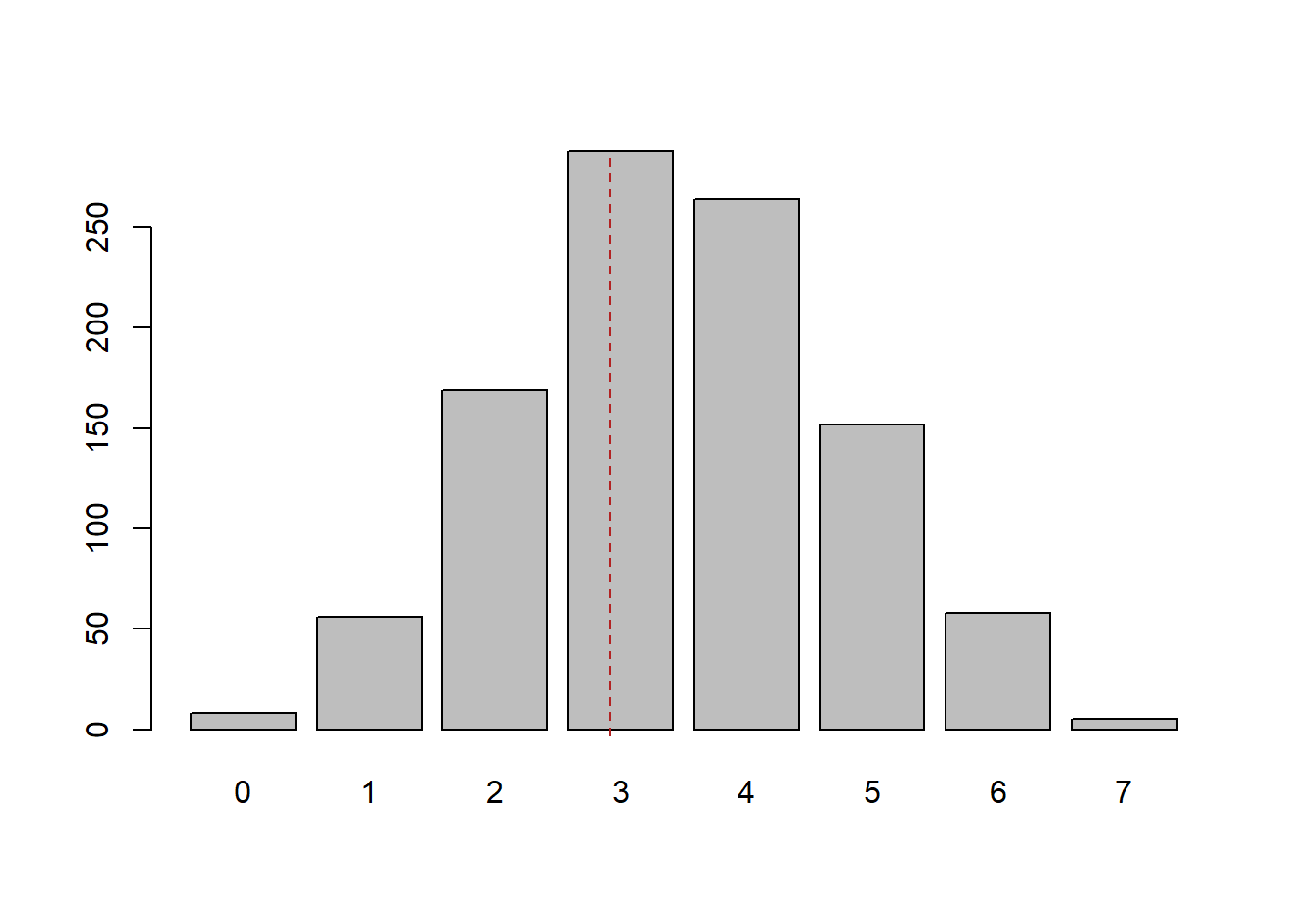
Now Lansing had only 3 wins in 7 films. We see that our repeated sampling from a world where wins and losses are equally likely that we get 3 wins in 7 films pretty frequently, approximately 25% of the time. Why does this help us? Well if what we are witnessing in reality is something that is likely to happen simply by random chance, we cannot discount the possibility that what we are observing is just random fluctuations! Put another way: there is so much noise inherent in just looking a stretch of 7 movies, this record cannot be distinguished from what might happen due to random chance.
But what if this were Lansing’s record:
\[ LLLLLLL \]
7 straight dud movies. Looking at the distribution of what occurred due to random chance, we see that in our 1000 simulations only 8 resulted in no wins. This is a very unlikely thing to happen simply due to random chance! If this was Lansing’s record I would be fine with concluding that she is actually a bad movie producer.
Now let’s consider another situation, let’s say we allowed Lansing to have a long (an absurdly long) career and allowed her to make 70 movies. Further, let’s imagine that in those 70 movies she has 30 hits. Notice that this is exactly the same proportion of “hits” as she got in the real world! But now the totals are scaled up.
Without thinking about math, would we be more or less confident that Lansing is a “bad” producer given this new information? My intuition is that we should be more confident at this point. We have more information that is consistent with her having more losses than wins at the box office.
We can modify the above code to look at what we can expect if wins and losses were just random, but instead look at 70 movies:
sample(c("W","L"), 70, replace=T)
#>  [1] "L" "L" "L" "L" "W" "L" "W" "L" "L" "W" "L" "L" "L" "W"
#> [15] "L" "W" "L" "W" "W" "L" "L" "L" "L" "L" "W" "L" "L" "W"
#> [29] "L" "W" "W" "W" "L" "L" "W" "L" "W" "W" "L" "L" "L" "L"
#> [43] "L" "L" "L" "L" "L" "L" "W" "W" "L" "L" "L" "W" "W" "W"
#> [57] "W" "W" "W" "W" "L" "W" "W" "L" "W" "L" "W" "W" "L" "W"
Again, we want to look at what is true in the long term about how frequently different numbers of wins happen due to random chance. So again we are just going to repeat this process many times, each time recording the number of wins:
number.wins <- NA
for(i in 1:1000){
  number.wins[i] <- sum(sample(c("W","L"), 70, replace=T)=="W")
}

table(number.wins)
#> number.wins
#>  22  23  24  25  26  27  28  29  30  31  32  33  34  35  36
#>   1   1   3  10  13  20  29  34  57  54  73  80  85  94 108
#>  37  38  39  40  41  42  43  44  45  46  47  50
#>  85  76  53  34  28  28  20   8   3   1   1   1
barplot(table(number.wins))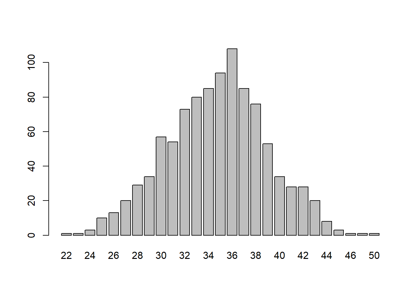
Before, we saw that by random choice we could expect to get 3 wins in 7 films around 25% of the time. But looking at this simulation we get 30 wins in 70 films only 6% of the time (60 of the 1000 trials). So it is relatively more rare for this outcome to happen simply due to random chance.
Going back to our question above, yes, we should be more confident about determining the underlying ability of Lansing when we have more information.
But, we were only able to do this because we were able to build a model of the underlying uncertainty in this situation, and to assess our information (i.e. 3 wins in 7 films or 30 wins in 70 films) against the backdrop of this underlying uncertainty.
A very similar example that we can extend the same reasoning to is a baseball hitter. I watch a fair amount of Phillies baseball, and commentators love to talk about the hot and cold streaks hitters go on, and to attribute those streaks to all manner of weird explanations (the weather, new bats, schedules, home-run derby effects….). Again, to understand whether something like a baseball hitter going into a prolonged slump (or hot-streak) is “real” we have to have a model of the underlying noise and uncertainty.
Last season, your friend and mine Bryce Harper, had 457 at-bats and got a hit 134 times, which equals a batting average of .293 (29.3%).
We can do something similar to above, and think about: if we flip a coin that comes up heads 29.3% of the time, how common are long streaks of too few heads or too few tails?
So first, let’s have R generate 450 at-bats where the probability of getting a hit is 29.3%:
set.seed(19104)
hits <- sample(c(1,0), 450, replace=T, prob=c(.293,.707))
mean(hits)
#> [1] 0.2822222
This represents a full season of at-bats, generated randomly.
Now three baseball games, which is about 10 at-bats, is a lot of baseball. Let’s look at what this hypothetical baseball player’s batting average is over all possible 10 at-bat stretches during the season we just generated.
avg <- NA
for(i in 1:441){
  end <- i+9
  avg[i]<- sum(hits[i:end])/10
}

plot(1:441,avg, type="l", main="A season of streaks", ylab="3-Game Batting Average",
     xlab="Games")
abline(h=.293, col="firebrick")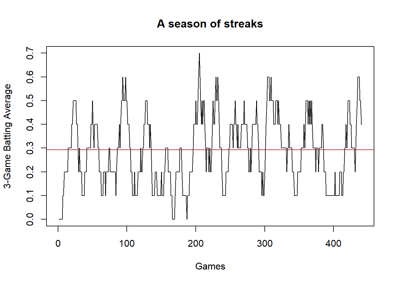
Each point in this line represents this hypothetical baseball players batting average over 3 games (10 at bats) over the course of the season. Notice how wildly variable it is! for long stretches of time it is very low or very high, just by random chance! There is nothing systematic creating these troughs and spikes. This is just what randomly generated data looks like.
So when we think about Bryce Harper having a 3 game slump (did he change socks? is the barometric pressure to high? did his wife move out of the house???) those slumps cannot be distinguished against what would happen just by random chance.
1.4 Back to the real world
So in some situations we can model the underlying uncertainty really easily and compare what we have observed what is likely to happen simply due to random chance. How does that help us in the real world when have a dataset like we had at the start of the lecture, one where we observe the degree to which Democrats and Republicans were going to restaurants?
Indeed, here is the real data:
library(rio)
dat <- import("https://github.com/marctrussler/IDS-Data/raw/main/SMPartisanRestaurant.Rds")
head(dat)
#>      restaurant democrat
#> 2256      FALSE    FALSE
#> 2258      FALSE     TRUE
#> 2262      FALSE    FALSE
#> 2290      FALSE    FALSE
#> 2291      FALSE     TRUE
#> 2292      FALSE    FALSE
There is data here on 845 thousand Americans from the spring and summer of 2020. Like the pretend data we had above, this includes information for each individual for whether they went to a restaurant, or not, and whether they are a Democrat, or not. (For simplicity I’ve taken independents out of this data, so people who are not Democrats are Republicans).
Let’s look at what this data says for our main research question: were Democrats less likely to go to a restaurant in the previous 7 days compared to Republicans?
mean(dat$restaurant)
#> [1] 0.122922
mean(dat$restaurant[dat$democrat==T])
#> [1] 0.05172414
mean(dat$restaurant[dat$democrat==F])
#> [1] 0.2060629
In our real sample around 20% of Republicans had been to a restaurant in the previous 7 days, while only 5% of Democrats had. So for this sample of people there is a clear association between partisanship and social distancing, with Democrats about 15 percentage points less likely to go to restaurants in the proceeding 7 days compared to Republicans.
But again, if we were to go out and get another sample we wouldn’t get exactly the same result. What’s to say that we wouldn’t get something like 2% difference in the next sample, or 15% in the other direction?
In the case of movie producers and baseball games it was relatively easy to model the inherent uncertainty and randomness in the situation to get a sense of “how strong of a signal do I need to have to overcome this noise?” In this situation there is no simple solution.
The good thing is that people have worked out, for a given estimate and a given sample size, exactly how much random noise can be expected due to differences from sample to sample. How this is worked out is a topic for another class, for right now it’s important for you to know that we have worked it out. For example, in the case of this difference in the two means, here is what the inherent randomness is expected to look like:
t <- t.test(dat$restaurant ~ dat$democrat)
values <- seq(-.005,.005,.00001)
plot(values, dnorm(values,sd=t$stderr), type="l")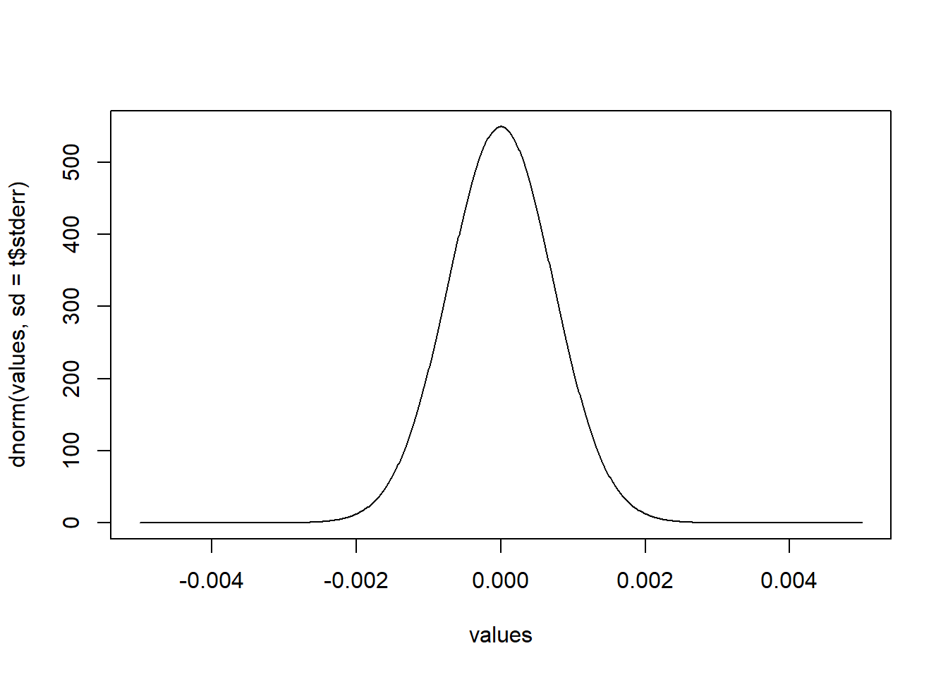
In this case, the expected noise is very small. We expect sampling to produce error around \(\pm .2%\) around the true value when we sample. So in this sample we got a difference of 15%, and if we were able to repeated re-sample we might expect differences of 14.8 or 14.6 or 15.2 or 15.4…. things around those numbers. As such: are we confident that the truth is not 0? Definitely! It would be extraordinarily weird to have this sample have a difference of 15 if the truth was that it was 0!
This number is really small in this case because we have so many people. In general, the more people we have in a sample, the less noise there is going to be in our estimate. This makes a lot of sense! In very small samples we might get very weird results, but as we scale up the weirdness in a sample reduces.
We express this concept of “how much noise can we expect there to be due to sampling” in the standard error. Later in this class we will express this more clearly (and if you take PSCI1801 you will know a lot about the standard error). For a single mean, we can get the standard error through this formula:
\[ \frac{sd(x)}{\sqrt{n}} \]
The standard error is calculated by dividing the standard deviation of what we have a sample of and dividing by square root of the sample size.
So, for example, if I had a poll of 1000 people for whether they are going to vote for Biden for re-election, or not:
We can find the standard error – again a measure of how much randomness can be expected due to repeated sampling – by dividing the standard deviation of this variable by the square root of the sample size (1000).
The standard error is about .016. That’s a fairly meaningless number to us right now, but let’s compare what the standard error is at different sample sizes, from 10 to 10000:
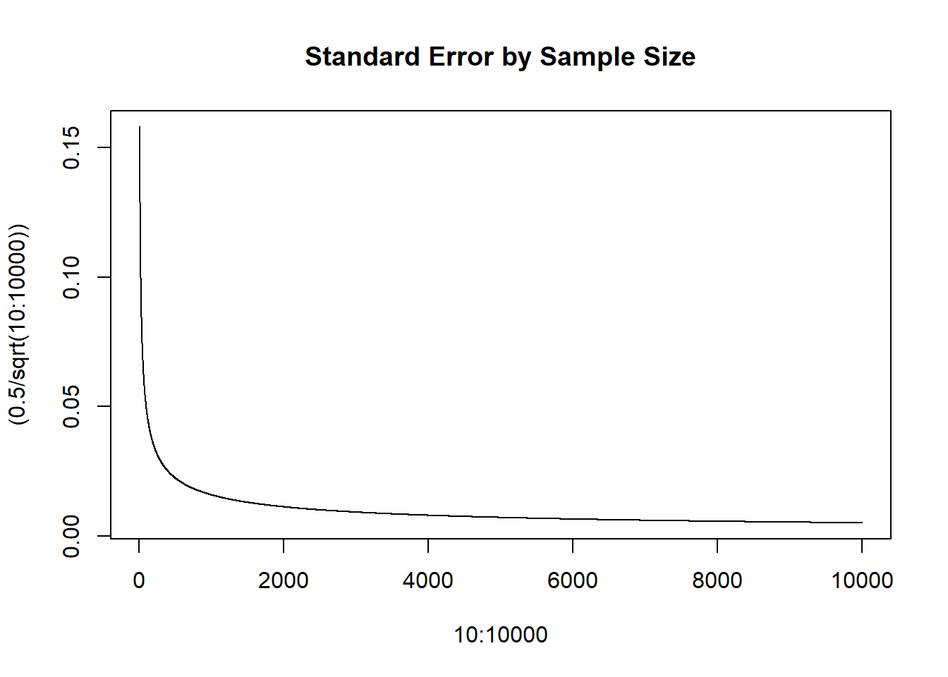
We see that the standard error decreases at a decreasing rate. That is to say: going from a a sample size of 10 to 100 matters a lot. Going from 100 to 1000 matters, but not as much. Going from 1000 to 10,000 matters, but not as much. More sample size gives us more precise estimates, but doing so gives diminishing returns.
1.5 Random Sampling (Think of the Soup)
Now all of the above assumed that the samples being taken were random samples of whatever it is that we are looking at. In the context of an election poll, traditional methods have you generate random phone numbers to call so that everyone in the US has an equally likely probability of being included. (Modern polling is slightly more complicated than this, which we can get into at a later date).
Random sampling is really what allows for the magic of statistics, and everything falls apart without it.
One clue to it’s importance comes from the equation for the standard error I presented above: \(\frac{sd(x)}{\sqrt{n}}\). For a mean, the amount of random noise that is to be expected is a function of how random our sample is (the standard deviation) and the sample size. One thing that is not in this equation is the size of the population.
This tells us, in other words, that a random sample of 1000 people has the same ability to tell us something about the population of Canada (33 million people) as it does for the population of the US (330 million) as it does for China (1.4 billion). As long as the sample is a random sample, the standard error for all three estimates will be the same.
How can this be? The best way to think about this is to think about soup. When you are making soup (I know you are all undergrads and don’t cook but you can imagine what it might be like to make soup) and you want to know if it tastes good, do you have to eat a huge bowl? No! You stir it up (randomization) and take just one spoonful to see how it tastes. It wouldn’t matter if you had a 1 quart or 30 quart pot, to see how it tastes you would still just take one spoonful (conditional on it being well mixed, which is the randomization part!)
1.6 The Big Picture
So what do I want you to know about statistics in this “not statistics” course?
Primarily, I want you to keep in mind that the things we are doing in this course – while vital! – are only one leg of the “data science” pyramid. We are going to learn a lot about loading, cleaning, manipulating, and presenting data. This work will be hard and I promise you will learn a lot of great skills. But these skills are fairly limited in isolation.
To this knowledge you will learn more about statistics. For right now, it’s enough to remember that every dataset we look at is one of an infinite number of datasets we could have. That means every thing we estimate is one of an infinite number of estimates we could have. To properly understand the estimates in our dataset we need a measure of how much noise is likely to occur based on these differences from sample-to sample.
We are going to talk about hypothesis testing down the road, which will give you some tools to use this information. But really, I encourage you to take further courses in statistics to properly understand this.