7 Review
The best way to review for the midterm will be to read the notes in this book and to carefully go through the problem set questions.
All of the questions in the problem sets are designed to be straight-forward applications of the class material. Oftentimes they are just class examples with re-named variables. Try to think about what different parts of the examples are doing. Try to edit things and see if they still work. For ex. an example makes deciles of population density, what if I made deciles of income instead?
The midterm questions will similarly be straight-forward applications of class examples. There may be cases where things are presented in a new form or combine concepts, but if you have a grasp of the in-class and problem set code there will be absolutely nothing surprising about the midterm.
My other tips for the midterm are: knit your rmarkdown often so you don’t get stuck at the end; read every question fully before starting; pay attention to extra information I’ve provided; pay attention to the words I use in the questions and how those words relate to the course material.
7.1 Review of Loops
acs <- rio::import("https://github.com/marctrussler/IDS-Data/raw/main/ACSCountyData.csv")Let’s try another use: What is the correlation of population density and percent commuting by car within each state?
To start with, what is the correlation for all the counties? I can get that via the cor function. When using this function I add the argument use="pairwise.complete" to tell R to only worry about cases where we have values for both variables.
cor(acs$population.density, acs$percent.car.commute, use="pairwise.complete")
#> [1] -0.3972397
Predictably, there is a negative correlation. As population density gets higher the percent of people using a car to commute gets lower.
But we might be curious if that correlation is different in different places. Maybe in the South where there is less investment in public transportation there will be a lower correlation?
How would we determine this correlation just for Alabama?
To do so I need to subset both variables:
cor(acs$population.density[acs$state.abbr=="AL"],
    acs$percent.car.commute[acs$state.abbr=="AL"])
#> [1] -0.2173754
Now put this in a loop and save the results to make graphing easier. In the same loop I’m also going to record what the Census region of each state is.
states <- unique(acs$state.abbr)
within.state.cor <- rep(NA, length(states))
census.region <- rep(NA, length(states))

for(i in 1:length(states)){
  within.state.cor[i] <- cor(acs$population.density[acs$state.abbr==states[i]],
                             acs$percent.car.commute[acs$state.abbr==states[i]],
                             use="pairwise.complete")
  #Why do I need to use unique here?
  census.region[i] <- unique(acs$census.region[acs$state.abbr==states[i]])
}

cbind(states,within.state.cor, census.region)
#>       states within.state.cor      census.region
#>  [1,] "AL"   "-0.2173754217653"    "south"
#>  [2,] "AK"   "0.306765991557315"   "west"
#>  [3,] "AZ"   "-0.0978290084303064" "west"
#>  [4,] "AR"   "0.105742290830552"   "south"
#>  [5,] "CA"   "-0.653978927772517"  "west"
#>  [6,] "CO"   "-0.0323180568609168" "west"
#>  [7,] "CT"   "-0.67901228835113"   "northeast"
#>  [8,] "DE"   "-0.886927793640683"  "south"
#>  [9,] "DC"   NA                    "south"
#> [10,] "FL"   "-0.259511132475236"  "south"
#> [11,] "GA"   "-0.389881360777326"  "south"
#> [12,] "HI"   "0.104587443762592"   "west"
#> [13,] "ID"   "0.169041971631012"   "west"
#> [14,] "IL"   "-0.685983927063127"  "midwest"
#> [15,] "IN"   "-0.199856034276139"  "midwest"
#> [16,] "IA"   "0.112736925807877"   "midwest"
#> [17,] "KS"   "0.243180720391614"   "midwest"
#> [18,] "KY"   "-0.294974731369198"  "south"
#> [19,] "LA"   "-0.615420891410212"  "south"
#> [20,] "ME"   "-0.197529385128518"  "northeast"
#> [21,] "MD"   "-0.756892276791218"  "south"
#> [22,] "MA"   "-0.889129033490708"  "northeast"
#> [23,] "MI"   "0.101872768345178"   "midwest"
#> [24,] "MN"   "-0.21613646697179"   "midwest"
#> [25,] "MS"   "0.029415641383925"   "south"
#> [26,] "MO"   "-0.201194925123038"  "midwest"
#> [27,] "MT"   "0.440739634106128"   "west"
#> [28,] "NE"   "0.175310702653679"   "midwest"
#> [29,] "NV"   "0.382886407964416"   "west"
#> [30,] "NH"   "0.310082253891291"   "northeast"
#> [31,] "NJ"   "-0.971976737123834"  "northeast"
#> [32,] "NM"   "0.0928055499087419"  "west"
#> [33,] "NY"   "-0.92500515456373"   "northeast"
#> [34,] "NC"   "-0.321664588357605"  "south"
#> [35,] "ND"   "0.475260375708698"   "midwest"
#> [36,] "OH"   "-0.251860957515806"  "midwest"
#> [37,] "OK"   "0.0301127777870135"  "south"
#> [38,] "OR"   "-0.475943129470221"  "west"
#> [39,] "PA"   "-0.842429745927983"  "northeast"
#> [40,] "RI"   "-0.320574836829983"  "northeast"
#> [41,] "SC"   "-0.55083792261745"   "south"
#> [42,] "SD"   "0.377332376588293"   "midwest"
#> [43,] "TN"   "-0.231591746107272"  "south"
#> [44,] "TX"   "-0.0698796287685257" "south"
#> [45,] "UT"   "0.0372286222243687"  "west"
#> [46,] "VT"   "-0.34891159979597"   "northeast"
#> [47,] "VA"   "-0.712800662117221"  "south"
#> [48,] "WA"   "-0.238851566121112"  "west"
#> [49,] "WV"   "-0.154420314967612"  "south"
#> [50,] "WI"   "-0.046798738079877"  "midwest"
#> [51,] "WY"   "0.400225390529855"   "west"
Looks good! Note that we don’t get a correlation for DC because there is only one “county” In DC.
What’s the best way to look at these? Our hypothesis said that states in different regions might have different correlations, so let’s visualize by region.
I’m going to make our results into a dataframe #And remove DC.
st.cor <- cbind.data.frame(states,within.state.cor, census.region)
st.cor <- st.cor[st.cor$states!="DC",]
I want to organize this dataset by region and then by correlation size. To do so we can add a second argument to order:
st.cor <- st.cor[order(st.cor$census.region, st.cor$within.state.cor),]
st.cor
#>    states within.state.cor census.region
#> 14     IL      -0.68598393       midwest
#> 36     OH      -0.25186096       midwest
#> 24     MN      -0.21613647       midwest
#> 26     MO      -0.20119493       midwest
#> 15     IN      -0.19985603       midwest
#> 50     WI      -0.04679874       midwest
#> 23     MI       0.10187277       midwest
#> 16     IA       0.11273693       midwest
#> 28     NE       0.17531070       midwest
#> 17     KS       0.24318072       midwest
#> 42     SD       0.37733238       midwest
#> 35     ND       0.47526038       midwest
#> 31     NJ      -0.97197674     northeast
#> 33     NY      -0.92500515     northeast
#> 22     MA      -0.88912903     northeast
#> 39     PA      -0.84242975     northeast
#> 7      CT      -0.67901229     northeast
#> 46     VT      -0.34891160     northeast
#> 40     RI      -0.32057484     northeast
#> 20     ME      -0.19752939     northeast
#> 30     NH       0.31008225     northeast
#> 8      DE      -0.88692779         south
#> 21     MD      -0.75689228         south
#> 47     VA      -0.71280066         south
#> 19     LA      -0.61542089         south
#> 41     SC      -0.55083792         south
#> 11     GA      -0.38988136         south
#> 34     NC      -0.32166459         south
#> 18     KY      -0.29497473         south
#> 10     FL      -0.25951113         south
#> 43     TN      -0.23159175         south
#> 1      AL      -0.21737542         south
#> 49     WV      -0.15442031         south
#> 44     TX      -0.06987963         south
#> 25     MS       0.02941564         south
#> 37     OK       0.03011278         south
#> 4      AR       0.10574229         south
#> 5      CA      -0.65397893          west
#> 38     OR      -0.47594313          west
#> 48     WA      -0.23885157          west
#> 3      AZ      -0.09782901          west
#> 6      CO      -0.03231806          west
#> 45     UT       0.03722862          west
#> 32     NM       0.09280555          west
#> 12     HI       0.10458744          west
#> 13     ID       0.16904197          west
#> 2      AK       0.30676599          west
#> 29     NV       0.38288641          west
#> 51     WY       0.40022539          west
#> 27     MT       0.44073963          west
And now graph this:
which(st.cor$census.region=="northeast")
#> [1] 13 14 15 16 17 18 19 20 21
which(st.cor$census.region=="south")
#>  [1] 22 23 24 25 26 27 28 29 30 31 32 33 34 35 36 37
which(st.cor$census.region=="west")
#>  [1] 38 39 40 41 42 43 44 45 46 47 48 49 50

plot(1:50, st.cor$within.state.cor, pch=16, ylim=c(-1,1), axes=F,
     xlab="",ylab="Correlation Population Density & Percent Car Commute")
abline(h=0, lty=2, col="gray80")
axis(side=2, at=seq(-1,1,.5), las=2)
axis(side=1, at=1:50, labels=st.cor$states, cex.axis=.5)
abline(v=c(12.5,21.5,37.5), lty=3)
text(c(6,17,29,44), c(1,1,1,1), labels = c("Midwest","Northeast","South","West"))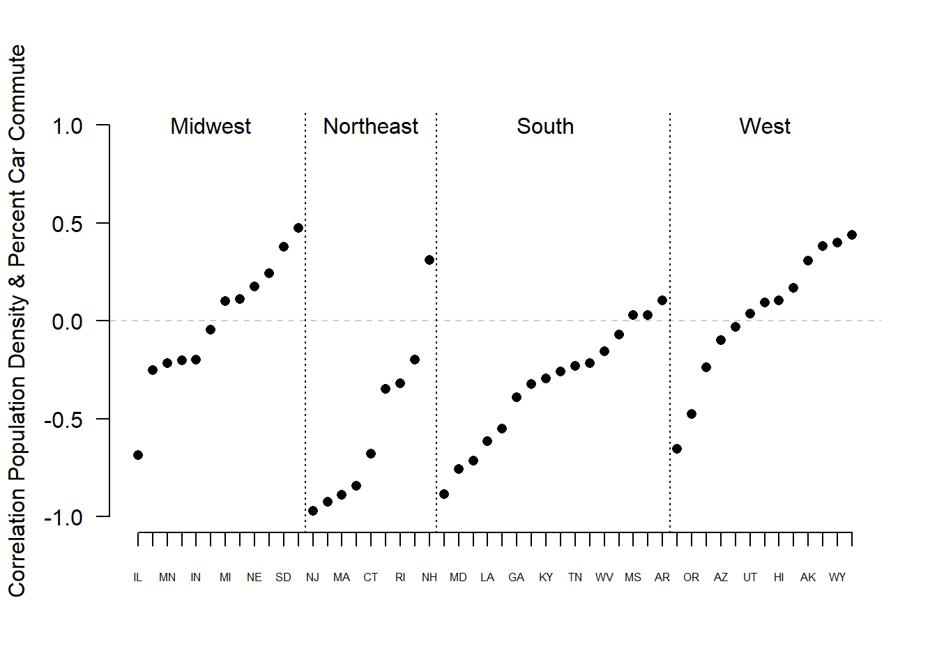
Here is a second double loop example:
What if we wanted to create a new ACS dataset that took the mean of all these variables for all of the states. So this same dataset, at the state rather than county level.
I’m going to load a fresh copy of ACS because i’ve created a bunch of stuff above:
acs <- rio::import("https://github.com/marctrussler/IDS-Data/raw/main/ACSCountyData.csv")
names(acs)
#>  [1] "V1"                      "county.fips"
#>  [3] "county.name"             "state.full"
#>  [5] "state.abbr"              "state.alpha"
#>  [7] "state.icpsr"             "census.region"
#>  [9] "population"              "population.density"
#> [11] "percent.senior"          "percent.white"
#> [13] "percent.black"           "percent.asian"
#> [15] "percent.amerindian"      "percent.less.hs"
#> [17] "percent.college"         "unemployment.rate"
#> [19] "median.income"           "gini"
#> [21] "median.rent"             "percent.child.poverty"
#> [23] "percent.adult.poverty"   "percent.car.commute"
#> [25] "percent.transit.commute" "percent.bicycle.commute"
#> [27] "percent.walk.commute"    "average.commute.time"
#> [29] "percent.no.insurance"
What we wantto do is to take averages for all of the variables from population to percent no insurance
We’d want to run code that looks like this, where we want to change both the state and the variable:
mean(acs[acs$state.abbr=="AL", "population"])
#> [1] 72607.16
Let’s create a list of the variables we want means for
vars <- names(acs)[9:28]
vars
#>  [1] "population"              "population.density"
#>  [3] "percent.senior"          "percent.white"
#>  [5] "percent.black"           "percent.asian"
#>  [7] "percent.amerindian"      "percent.less.hs"
#>  [9] "percent.college"         "unemployment.rate"
#> [11] "median.income"           "gini"
#> [13] "median.rent"             "percent.child.poverty"
#> [15] "percent.adult.poverty"   "percent.car.commute"
#> [17] "percent.transit.commute" "percent.bicycle.commute"
#> [19] "percent.walk.commute"    "average.commute.time"
And we know how to make a list of states:
states <- unique(acs$state.abbr)
states
#>  [1] "AL" "AK" "AZ" "AR" "CA" "CO" "CT" "DE" "DC" "FL" "GA"
#> [12] "HI" "ID" "IL" "IN" "IA" "KS" "KY" "LA" "ME" "MD" "MA"
#> [23] "MI" "MN" "MS" "MO" "MT" "NE" "NV" "NH" "NJ" "NM" "NY"
#> [34] "NC" "ND" "OH" "OK" "OR" "PA" "RI" "SC" "SD" "TN" "TX"
#> [45] "UT" "VT" "VA" "WA" "WV" "WI" "WY"
How can we take advantage of the loop functionality to index both of these things?
Let’s try this way first (THIS IS WRONG)
i<- 1
mean(acs[acs$state.abbr==states[i], vars[i]])
#> [1] 72607.16
What would happen if we ran this code in a loop?
That doesn’t work! We are telling R to get the mean of the first state for the first variable, then the mean of the second state for the second variable, mean of the third state for the third variable…
mean(acs[acs$state.abbr==states[1], vars[1]])
#> [1] 72607.16
mean(acs[acs$state.abbr==states[2], vars[2]])
#> [1] 7.880517
Instead we need to say: Ok, R. Start with the first variable (population). For this variable, loop through all of the states. Once you’re finished with that, move on to the second variable and loop through all of the states again.
We want to do something like this, where we are preserving the loop that already works, and thenprogressively working through each variable:
for(i in 1:length(states)){
  mean(acs[acs$state.abbr==states[i], "population"], na.rm=T)
}


for(i in 1:length(states)){
  mean(acs[acs$state.abbr==states[i], "population.density"], na.rm=T)
}


for(i in 1:length(states)){
  mean(acs[acs$state.abbr==states[i], "percent.senior"], na.rm=T)
}
To do so, we want to set up an “outer” loop that moves through the variables
We get something like this:
for(j in 1: length(vars)){
  for(i in 1:length(states)){
    mean(acs[acs$state.abbr==states[i], vars[j]], na.rm=T)
  }
}
Notice that we are now indexing by two objects: i & j. i is indexing states, j is indexing variable names.
So R will start the outside loop with j=1, it will then start the inside loop with i=1, and keep running that inside loop until i=51. Then it will go back to the start of the outside loop and make j=2…
But where are we going to save these estimates? We now have to save them in a matrix with both rows and columns.
Think about what we want to do here: we want to
for(i in 1:length(states)){
  state.demos[i,1] <-  mean(acs[acs$state.abbr==states[i], vars[1]], na.rm=T)
}


for(i in 1:length(states)){
  state.demos[i,2] <-  mean(acs[acs$state.abbr==states[i], vars[2]], na.rm=T)
}


for(i in 1:length(states)){
  state.demos[i,3] <-  mean(acs[acs$state.abbr==states[i], vars[3]], na.rm=T)
}
Notice how the numbers are increasing the same way on the left and right side of the assignment operator
We need to tell R where to save each mean, with the correct row and column:
for(j in 1: length(vars)){

  for(i in 1:length(states)){
    state.demos[i,j] <-  mean(acs[acs$state.abbr==states[i], vars[j]], na.rm=T)
  }

}
It’s easy, then, to combine this matrix with the state names we have saved, and to use the vars vector to create labels.
state.demos <- cbind.data.frame(states,state.demos)

names(state.demos)[2:21] <- vars
Note, additionally, that we could have organized that loop in the opposite way, making the outer loop index through states, and the inner loop index through variables:
This gives the exact same result:
state.demos2 <- matrix(NA, nrow=length(states), ncol=length(vars))


for(i in 1: length(states)){

  for(j in 1:length(vars)){
    state.demos2[i,j] <-  mean(acs[acs$state.abbr==states[i], vars[j]], na.rm=T)
  }

}

state.demos2 <- cbind.data.frame(states,state.demos2)

names(state.demos2)[2:21] <- vars
WARNING: THIS ISN’T ACTUALLY HOW YOU WOULD FIND OUT THE AVERAGE FOR EACH STATE. Just looking at the mean of county values for each of these variables assumes each county is of the same population. They obviously are not!
7.2 If statements
The conditional statements we’ve worked with so far have evaluated our data to say, if this condition holds in this row, take this action. Sometimes we want to extend this and say, if a certain condition holds, Run this code
We can do this via if statements. Similar to when we do this for a single line of code, we start with a logical statment – a statement that produces a single T or F, and then R will only run the code if the statement is True.
So for example:
operation <- "add"
if (operation == "add") {
  print("I'm going to add:")
  4+4
}
#> [1] "I'm going to add:"
#> [1] 8
But if we do the following it won’t work:
operation <- "multiply"

if (operation == "add") {
  print("I'm going to add:")
  4+4

}
Nothing happened here, and that is by design. R thought: in order for me to run this code chunk,this logical statement has to be True, it’s not, so I’ll skip it.
But if we set up a second if statement it will work:
if (operation == "multiply") {
  print("I'm going to multiply:")
  4*4
}
#> [1] "I'm going to multiply:"
#> [1] 16
We can even run both at the same time and only get the one that evaluates as True.
operation <- "multiply"
if (operation == "add") {
  print("I'm going to add:")
  4+4

}
if (operation == "multiply") {
  print("I'm going to multiply:")
  4*4

}
#> [1] "I'm going to multiply:"
#> [1] 16

operation <- "add"

if (operation == "add") {
  print("I'm going to add:")
  4+4

}
#> [1] "I'm going to add:"
#> [1] 8
if (operation == "multiply") {
  print("I'm going to multiply:")
  4*4
}
Right now our if statement says: if condition is True, run code, if it’s not, do nothing. But often times we want to say: if condition is True, run code, if it’s not, run this other code.We can accomplish this by adding an “else”
if(2+2==4){
  print("code chunk 1")
} else {
  print("code chunk 2")
}
#> [1] "code chunk 1"

if(2+2==5){
  print("code chunk 1")
} else {
  print("code chunk 2")
}
#> [1] "code chunk 2"
So if we wanted a chunk of code that adds if we tell it to, but otherwise multiplies:
operation <- "add"

if (operation == "add") {
  print("I'm going to add:")
  4+4

} else {
  print("I'm going to multiply:")
  4*4
}
#> [1] "I'm going to add:"
#> [1] 8

operation <- "subtract"

if (operation == "add") {
  print("I'm going to add:")
  4+4

} else {
  print("I'm going to multiply:")
  4*4
}
#> [1] "I'm going to multiply:"
#> [1] 16
The nice thing about these is they are infinitely stackable using else if ()
operation  <- "subtract"

if (operation == "add") {
  print("I'm going to add:")
  4+4

} else if (operation=="multiply") {
  print("I'm going to multiply:")
  4*4
} else {
  print("Please enter a valid operator.")
}
#> [1] "Please enter a valid operator."
Where is this sort of thing helpful? This is a bit of a “you’ll know it when you see it” situation. Where I use them most is inside loops. For example in election work I am often loading in many snapshots of data from across an election night, and I might only run certain functions when a state has reached a certain threshold of completeness.
Here is an example of where it might be helpful. Here are the 2020 presidential election results by county:
pres <- rio::import("https://github.com/marctrussler/IDS-Data/raw/main/CountyPresData2020.Rds")What if I want to record the winning margin in each state. That is: regardless of whether Trump or Biden carried the state, how much did they win by?
First, let’s write code that finds the dem and rep margin in each state:
head(pres)
#>   state county fips.code biden.votes trump.votes
#> 1    AK   ED 1     02901        3477        3511
#> 2    AK  ED 10     02910        2727        8081
#> 3    AK  ED 11     02911        3130        7096
#> 4    AK  ED 12     02912        2957        7893
#> 5    AK  ED 13     02913        2666        4652
#> 6    AK  ED 14     02914        4261        6714
#>   other.votes
#> 1         326
#> 2         397
#> 3         402
#> 4         388
#> 5         395
#> 6         468
pres$total.votes <- pres$biden.votes + pres$trump.votes + pres$other.votes

state <- unique(pres$state)
dem.perc <- NA
rep.perc <- NA

i <- 1
for(i in 1:length(state)){
  dem.perc[i] <- sum(pres$biden.votes[pres$state==state[i]])/ sum(pres$total.votes[pres$state==state[i]])
  rep.perc[i] <- sum(pres$trump.votes[pres$state==state[i]])/ sum(pres$total.votes[pres$state==state[i]])

}
results <- cbind.data.frame(state, dem.perc, rep.perc)
Pretty good! But to also calculate the winning margin in each state our code will need to be different dependent on the code of those two columns. Specifically, if the dem is the winner then the winning margin is dem-rep but if the rep is the winner then the winning margin is rep-dem. We can accomplish this via an if statement:
state <- unique(pres$state)
dem.perc <- NA
rep.perc <- NA
winner.margin <- NA
i <- 1
for(i in 1:length(state)){
  dem.perc[i] <- sum(pres$biden.votes[pres$state==state[i]])/ sum(pres$total.votes[pres$state==state[i]])
  rep.perc[i] <- sum(pres$trump.votes[pres$state==state[i]])/ sum(pres$total.votes[pres$state==state[i]])

  if(dem.perc[i]>rep.perc[i]){
    winner.margin[i] <- dem.perc[i]- rep.perc[i]
  } else {
    winner.margin[i] <- rep.perc[i]-dem.perc[i]
  }

}
results <- cbind.data.frame(state,dem.perc, rep.perc, winner.margin)
results <- results[order(results$winner.margin),]
Why would this have been wrong?
state <- unique(pres$state)
dem.perc <- NA
rep.perc <- NA
winner.margin <- NA
i <- 1
for(i in 1:length(state)){
  dem.perc[i] <- sum(pres$biden.votes[pres$state==state[i]])/ sum(pres$total.votes[pres$state==state[i]])
  rep.perc[i] <- sum(pres$trump.votes[pres$state==state[i]])/ sum(pres$total.votes[pres$state==state[i]])

  if(dem.perc[i]>rep.perc[i]){
    winner.margin[i] <- dem.perc[i]- rep.perc[i]
  }
    winner.margin[i] <- rep.perc[i]-dem.perc[i]

}
results <- cbind.data.frame(state,dem.perc, rep.perc, winner.margin)
results <- results[order(results$winner.margin),]