10 Hypothesis Tests
Now that we have a good sense of how to use R to load, manipulate, and present data, we are going to move on to creating and better understanding output.
The first thing we are going to talk through is “hypothesis testing” which a broad term for trying to understand the degree to which we can use a sample of data to understand the broader world. In the first half of this chapter we will talk about the logic of hypothesis testing and in the second half we will discuss how to implement hypothesis testing in R.
This is a relatively gentle introduction to a big topic. Hypothesis testing is actually the point of statistics and the depth you can get into this is bottomless. PSCI-1801 is a class entirely focused on better understanding hypothesis tests.
10.1 Review of “What is Data?”
At the start of the class we had a lecture on “What is Data?”
The purpose of that chapter was to have you think broadly about what we should be thinking about when we are looking at a dataset. The big risk with this course is that we spend so much time thinking about how to manipulate data on our computer that we forget about the big picture.
The “Big Picture” is that we are interesting in using our data to make inferences about the broader world. Critical to this is that every dataset we look at is one of an infinite number of datasets we could have. This is best conceptualized in the survey-research framework, where we can consider how there could be an infinite number of samples of, say, 1000 Americans. This is also true, however, of data like the ACS or the Census. Because there are an infinite number of datasets, it also means the everything we estimate is one of an infinite number of estimates we could have. To properly understand the estimates in our dataset we need a measure of how much noise is likely to occur based on these differences from sample-to sample.
The science of statistics is the process of measuring random noise and trying to infer properties of some real “truth” given that underlying uncertainty.
Critically, the random noise than can be expected is not a totally weird and unknowable thing. Instead, the random noise that occurs when estimating something across many samples is actually quite predictable. We call the distribution of all possible estimates across all possible samples the “sampling distribution” and it is the most critical component of statistics.
For example: we can consider the sampling distribution for the number of heads you get in the flip of 7 coins. Every time we flip 7 coins we get a different number of heads, but not all possibilities are equally likely:
#(I will explain set.seed() below)
set.seed(2107)
num.heads <- rep(NA, 10000)

coin <- c(0,1)

for(i in 1:1000){
  num.heads[i] <- sum(sample(coin, 7, replace=T))
}
prop.table(table(num.heads))
#> num.heads
#>     0     1     2     3     4     5     6     7
#> 0.009 0.053 0.175 0.266 0.265 0.174 0.049 0.009
barplot(prop.table(table(num.heads)), main="Sampling Distribution of  Num. Heads in 7 Flips")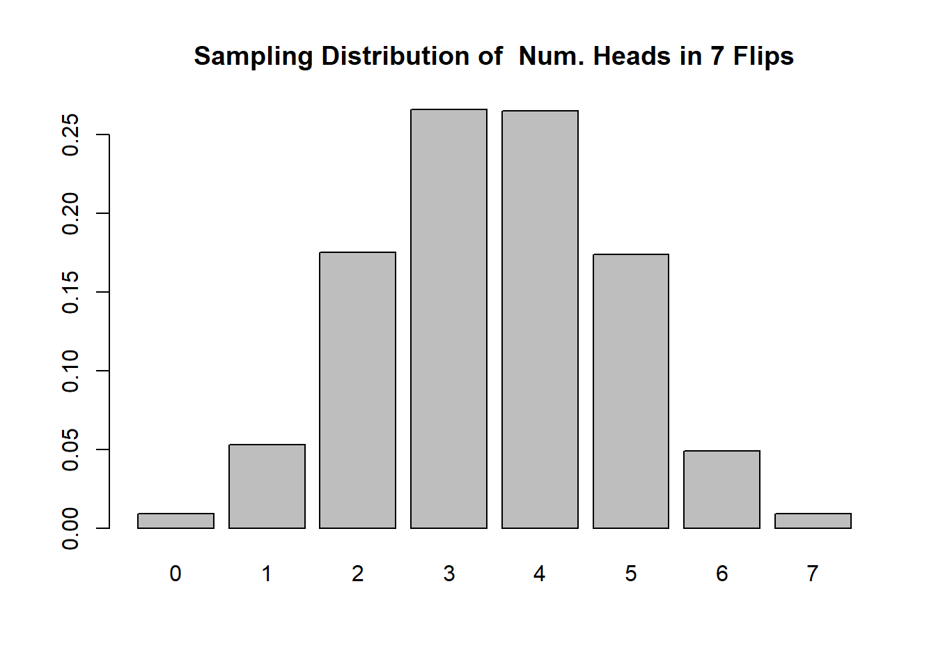
Here we are drawing the sampling distribution after repeating this sampling 1000 times, but we can also think about this in reverse: this is the distribution that the number of heads is drawn from whenever we flip a coin 7 times. If we think about what we are likely to get for the number of heads the next time we flip a coin 7 times, this sampling distribution represents all of the possibilities and their associated likelihood: ie it’s likely we will get 3 or 4 heads; it’s very unlikely we will get 0 or 7 heads etc.
10.2 Hypothesis Testing
To move from this informal understanding of randomness to a more formal method of hypothesis testing, we have to think about the type of question we want to ask, and how we can make use of the sampling distribution to answer those questions.
Above we generated the sampling distribution for the number of heads when flipping a coin 7 times. We saw that we get 3 or 4 heads around 27.5% of the time, for example.
Now imagine I give you a coin and ask you to flip it 7 times. After those 7 times, I want you to infer something about the truth in terms of how often this coin comes up heads.
So you do the flipping and you get the following result:
c(0,0,0,1,0,1,0)
#> [1] 0 0 0 1 0 1 0
We flipped the coin 7 times and it came up heads twice.
What can we infer about the truth of the coin we have flipped? This coin has a true percentage of the time it comes up heads, can we make a guess at precisely what that percentage is?
Well, we could guess that the truth is that the coin comes up heads \(2/7\) of the time, but that’s a hard thing to sustain. We know that every time we flip 7 coins we are going to get a slightly different answer and our method cannot be “Our belief about the truth is whatever we get in the sample.”
Instead of trying to same something definitive about the truth of how often the coin comes up heads, we are going to re-frame the type of question we are asking.
To do a hypothesis test, we are going to assume that the truth about the coin is that it comes up heads 50% of the time. From there, we are going to ask: if this is the truth, how likely is it to get the result that we did?
This is a helpful thing to do because we already have the sampling distribution for a fair coin. We have a good sense of what the distribution of estimates will be if we were to flip 7 coins a large number of times. As a reminder, here was the relative frequency of the outcomes:
prop.table(table(num.heads))
#> num.heads
#>     0     1     2     3     4     5     6     7
#> 0.009 0.053 0.175 0.266 0.265 0.174 0.049 0.009
In this table, which was generated using a fair coin, we see that around 17.5% of the time we get 2 heads in 7 flips of a fair coin.
So: if we assume that this coin is fair, is it likely or unlikely to get 2 heads in 7 flips? It’s relatively unlikely but still happens a good proportion of the time. Because an outcome likes this happens a good amount of the time with a fair coin we cannot exclude the possibility that this is a fair coin.
To put this more formally, there are 4 steps in hypothesis testing
Calculate a statistic in our sample.
State the null hypothesis.
Estimate the distribution of the statistic if the null were true in an infinite number of samples. (The sampling distribution).
Determine whether our particular result is unlikely or likely if the null were true given the sampling distribution.
To apply those steps to the coin flipping example we did:
The number of heads was 2/7
The null hypothesis is that the coin is fair, and comes up heads 50% of the time.
We used R to simulate flipping a coin 7 times and built the distribution of what that would look like.
We saw that 2/7 heads happens pretty often with a fair coin, so we decided to not reject the null hypothesis.
10.3 Applying that logic to “real” data
That’s all well and good for something like a coin flip where we can easily build a sampling distribution through simulation in R, but what about the real world? If we are thinking about a survey sample, we can’t go out and do 1000 more surveys to get a distribution of estimates. How can we think about applying null hypothesis testing to this situation?
Consider a situation where we do a survey of 300 people on whether they support Joe Biden or not.
I’m going to make up some data to simulate this situation.
In this first example the “truth” is going to be that Americans are ambivalent about the President, such that 50% of them support him and 50% of them oppose him
truth <- c(rep(1,50), rep(0,50))

#And make a population from that, which is 1 million people.
set.seed(1235)
pop <- sample(truth, 100000, replace = T)
summary(pop)
#>    Min. 1st Qu.  Median    Mean 3rd Qu.    Max.
#>  0.0000  0.0000  1.0000  0.5012  1.0000  1.0000
We are going to take one sample of 300 people
#Now in the real world, we would get exactly one sample:
set.seed(2107)
prime.sample <- sample(pop, 300)
head(prime.sample)
#> [1] 1 1 0 0 1 1
mean(prime.sample)
#> [1] 0.4633333
Let me stop here and explain the command set.seed(). There are a number of commands in R that produce “random” output. One of these commands is sample, such that every time you run it you get a different answer:
sample(1:1000,1)
#> [1] 824
sample(1:1000,1)
#> [1] 637
sample(1:1000,1)
#> [1] 268
sample(1:1000,1)
#> [1] 780
Computers can’t actually generate random things, and the way that it works (to simplify) is that it has a long list of random numbers stored that it references to generate a random outcome. (Before the age of personal computing you could go to the library and get a printed book of random numbers). If we tell R where to start in its list of random numbers, however, we will always generate the same output.
set.seed(1)
sample(1:1000,1)
#> [1] 836
sample(1:1000,1)
#> [1] 679
sample(1:1000,1)
#> [1] 129
set.seed(1)
sample(1:1000,1)
#> [1] 836
sample(1:1000,1)
#> [1] 679
sample(1:1000,1)
#> [1] 129
set.seed(1)
sample(1:1000,1)
#> [1] 836
sample(1:1000,1)
#> [1] 679
sample(1:1000,1)
#> [1] 129
This is helpful when i’m building notes because it means I get the same results everytime I knit this file. You can also make use of the set.seed() function in your problem sets so you get the same answer every time you knit.
Back to our sample of 300:
head(prime.sample)
#> [1] 1 1 0 0 1 1- Calculate a statistic in our sample.
We want to know the proportion of people who support Biden, that is:
mean(prime.sample)
#> [1] 0.4633333
46.3% of people in the sample support Joe Biden.
- State the null hypothesis.
The null hypothesis can be anything, but for right now a good one is that the true level of support for Biden is 50%, which would be half of all people liking him or half of all people not liking him. (Other null hypotheses might be: is Biden’s appproval 0? is Biden’s support different from Trump’s when he left office (38%)?)
- Estimate the distribution of the statistic if the null were true in an infinite number of samples. (The sampling distribution).
Now here we explicitly have the population, which we would not actually have in the real world. What’s more, we actually know in this case that true level of support for Biden in the population is 50%. As such, if we just repeatedly sample and take means, we will build the sampling distribution under the null hypothesis:
samp.dist <- NA

for(i in 1:10000){
  samp.dist[i] <- mean(sample(pop,300))
}

head(samp.dist)
#> [1] 0.5033333 0.4500000 0.5233333 0.4666667 0.4800000
#> [6] 0.4666667
This gives us 10,000 means from 10,000 samples of 300 people, each a little bit different. Here is what the distribution of those samples look like:
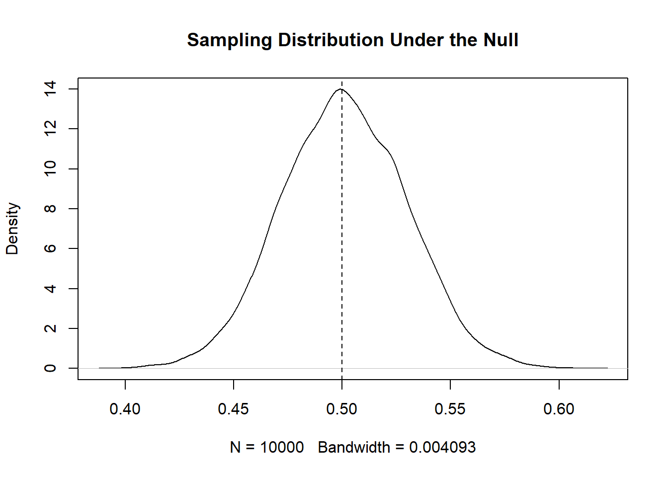
This is what get’s produced when we take a sample of 300 people 10,000 times and take the mean. But like above, we can also think about this distribution of describing the relative likelihood of getting different means in samples of 300 people. 50% is the most likely, 45% and 55% are less likely than that, almost never do we get something like 40% and 60%.
- Determine whether our particular result is unlikely or likely if the null were true given the sampling distribution.
Now we can compare our actual result in our “prime” sample to this sampling distribution:
plot(density(samp.dist), main="Sampling Distribution Under the Null")
abline(v=.5, lty=2)
abline(v=mean(prime.sample), lty=2, lwd=2, col="firebrick")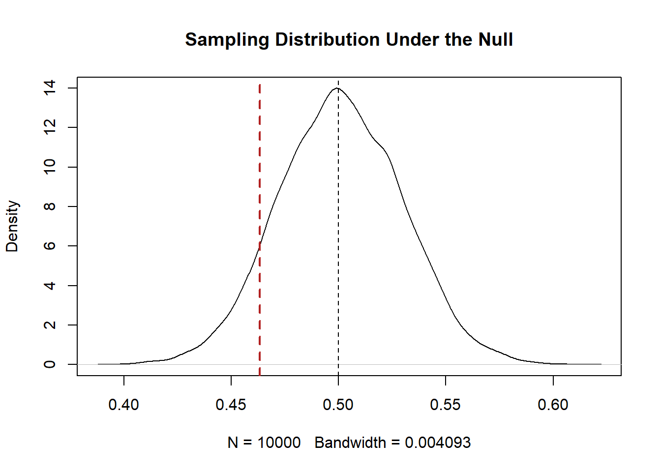
Is it likely or unlikely that we would get a result like this if the truth was 50%? Just eyeballing it, I would say that it is pretty likely. Means of 46% are generated with pretty regular frequency. In this case we would fail to reject the null hypothesis that the true level of Biden support is 50%
That’s all fine, but we’ve all noticed that a critical part of this process was that I pretended I could get 10,000 more samples of 300 people and use that to calculate a sampling distribution. In the real world I obviously cannot do that!
So how can we possibly draw a sampling distribution – the distribution of all possible estimates if we repeatedly sampled an infinite number of times – in the real world?
The answer to this question is somewhat complicated so I’m going to give you a watered down version here. For the full version you can take PSCI1801.
We can see that the sampling distribution looks like a bell curve: it is is symmetrical and declines from it’s peak in a bell-like pattern. In statistics we refer to bell-shaped distribution as a “normal” distribution. (Though not all bell shaped distributions are perfectly “normal” shaped).
A critical thing about normal distributions is that they are defined by their standard deviations. If I know the standard deviation of a normal distribution I can draw it exactly.
The standard deviation of all of our estimates is:
sd(samp.dist)
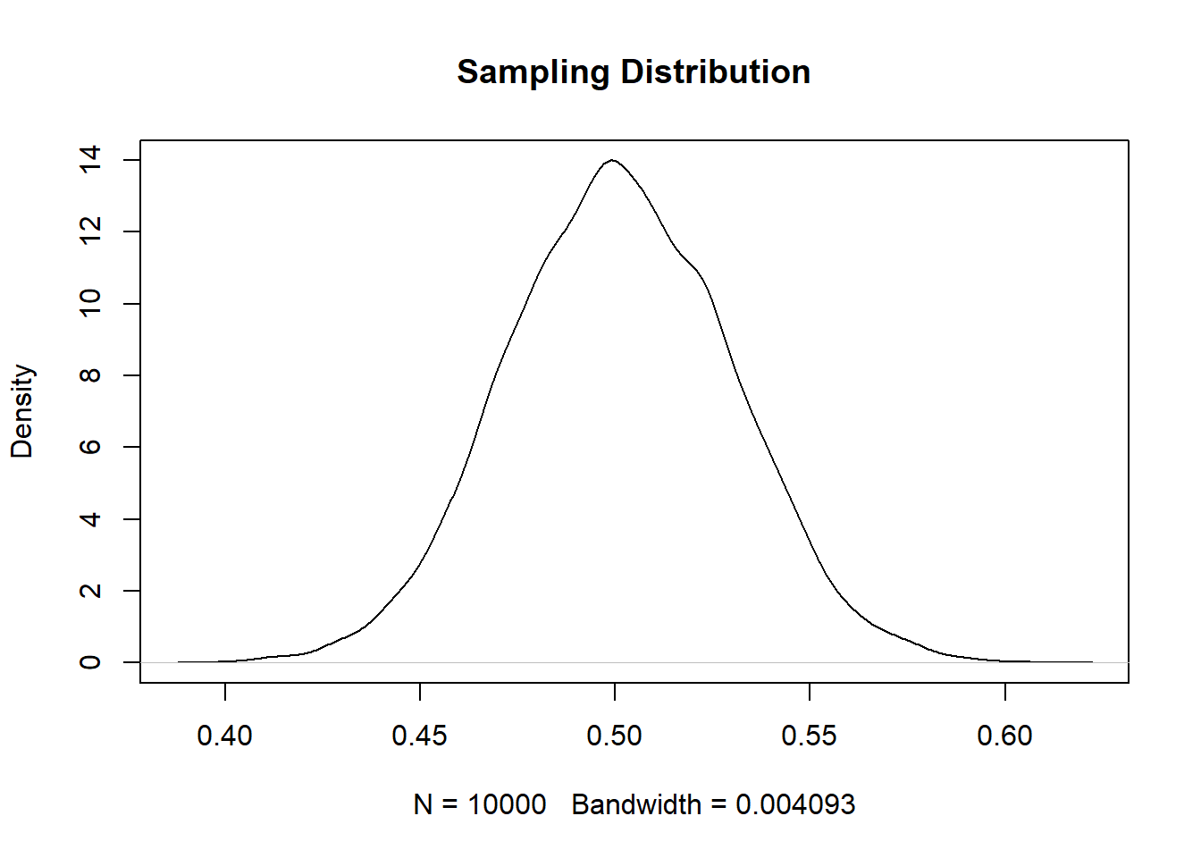
#> [1] 0.0286915If I take that and put it into a function that draws normal distributions:
eval <- seq(.4,.6,.001)
plot(density(samp.dist), main="Sampling Distribution")
points(eval,dnorm(eval, mean=.5, sd=sd(samp.dist)), col="magenta", type="l")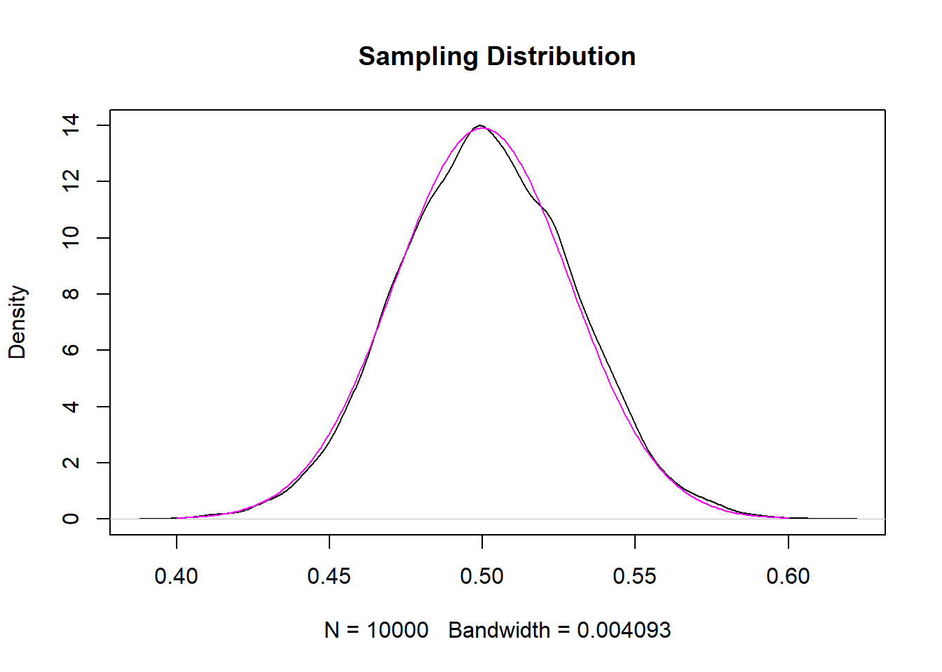
The resulting distribution is the “perfect” version of what we got from randomly sampling.
Now this standard deviation of the sampling distribution has a special name: the standard error. The standard error is the most important component of frequentist statistics so it is worth commiting it’s definition to memory: the standard error is the standard deviation of the sampling distribution.
The reason that it is important is because if we can estimate the standard error than we know exactly what the sampling distribution will look like! Again, above I showed that all we need to do to draw a normal distribution is know it’s standard deviation. So if we know the standard error (the standard deviation of the sampling distribution) we can draw a normal distribution for any null hypothesis we want.
Here is the last step: for many of the estimates that we care about, statistics has worked on the equations to estimate the standard error using information contained only in one sample.
Above, we found that the standard error of our repeatedly sampled estimate of Biden support in samples of 300 people was approximately .028.
Statistics has worked out that we can estimate the standard error of the sample mean by dividing the standard deviation of our sample by the square root of the sample size:
It’s almost exactly the same.
To re-iterate what I’m showing here: We initially built a sampling distribution by drawing repeated samples of 300 people from the population and calculating Biden’s percent approval in each of them. This step is impossible in the real world. We can’t get 1000 samples of 300 people. We took the standard deviation of this distribution and found the standard error was 0.028. But, the exact same number can be generated just with information from one sample, using the equation that was provided (the standard deviation of the sample divided by the square root of the number of observations.)
After all of this, here’s what we actually do to perform a hypothesis test:
t.test(prime.sample, mu=.5)
#>
#>  One Sample t-test
#>
#> data:  prime.sample
#> t = -1.2715, df = 299, p-value = 0.2045
#> alternative hypothesis: true mean is not equal to 0.5
#> 95 percent confidence interval:
#>  0.4065824 0.5200843
#> sample estimates:
#> mean of x
#> 0.4633333
We have to give the t.test() function our null hypothesis (default value is 0), but otherwise it did the rest.
We can see that it calculated the same standard error:
t.test(prime.sample, mu=.5)$stderr
#> [1] 0.02883789
The “t-value” is how many standard errors our estimate is from the null hypothesis:
(.5 - mean(prime.sample))/0.028
#> [1] 1.309524
The p-value is the most critical value: it represents the probability of obtaining a result as extreme as we did if the null hypothesis was true. In this case that probability is around 20%. In general, we fail to reject the null hypothesis if this value is under 5%.
10.4 Applying Hypothesis Testing
The previous section talked about hypothesis testing theoretically, but now we want to discuss how we can apply hypothesis testing in the real world.
To do so we are going to work with data we collected at NBC in September of 2020. This is data on 55 thousand Americans:
sm.dat <- rio::import("https://github.com/marctrussler/IDS-Data/raw/main/SMData.Rds")
head(sm.dat)
#>         trump.approve dem rep      party
#> 1207838             1   0   0       <NA>
#> 1223744             0   1   0   Democrat
#> 1229482             1   0   1 Republican
#> 1232667             0   1   0   Democrat
#> 1237784             0   1   0   Democrat
#> 1238590             1   0   1 Republican
The things we have in this data is an indicator for whether the respondent approves of Trump(1) or not (0), and then the respondents party coded a couple of different ways.
What sort of hypothesis test might we want to run on these data?
I propose this:
Data: Whether Americans approve (1) or not (0) of Donald Trump in September.
Question: Do Americans have a positive or negative view of the president?
Statistic: % Approve of Trump.
Null Hypothesis: American are entirely ambivalent about the president. % Approve == 50/%.
The four step hypothesis test we discussed last time is:
- Calculate a statistic in our sample.
This is very easy, we are just taking the mean of this variable:
mean(sm.dat$trump.approve, na.rm=T)
#> [1] 0.4066907
In this sample approximately 41% of people approve of Trump.
- State the null hypothesis.
As stated above, our null hypothesis is: American are entirely ambivalent about the president. Mathematically: \(\% Approve = 50\%\).
- Estimate the distribution of the statistic if the null were true in an infinite number of samples. (The sampling distribution).
This is the critical step of hypothesis testing, but now we are in the real world. To understand how much variability there is in our estimates we can’t do 1000 more samples of 55k people!
Instead, we are going to rely on the fact that there is a known equation to determine the standard error of a sample mean.
To refresh: what is the standard error? The standard error is the standard deviation of the sampling distribution. This value is critical because the sampling distribution is normally distributed, and to draw a normal distribution what you need is it’s standard deviation.
For a sample mean the standard error is equal to \(sd(x)/\sqrt{n}\).
se <- sd(sm.dat$trump.approve, na.rm=T)/sqrt(length(sm.dat$trump.approve[!is.na(sm.dat$trump.approve)]))
se
#> [1] 0.002107758
A very small number!
Let’s visualize that as a normal distribution (I don’t expect you to know this code):
prime.sd <- dnorm(seq(.4,.6,.001), mean=.5, sd=se)

plot(seq(.4,.6,.001), prime.sd, type="l")
abline(v=.5,lty=2, lwd=2)
legend("topright", c("Null Hypothesis"), lty=c(2), lwd=c(2))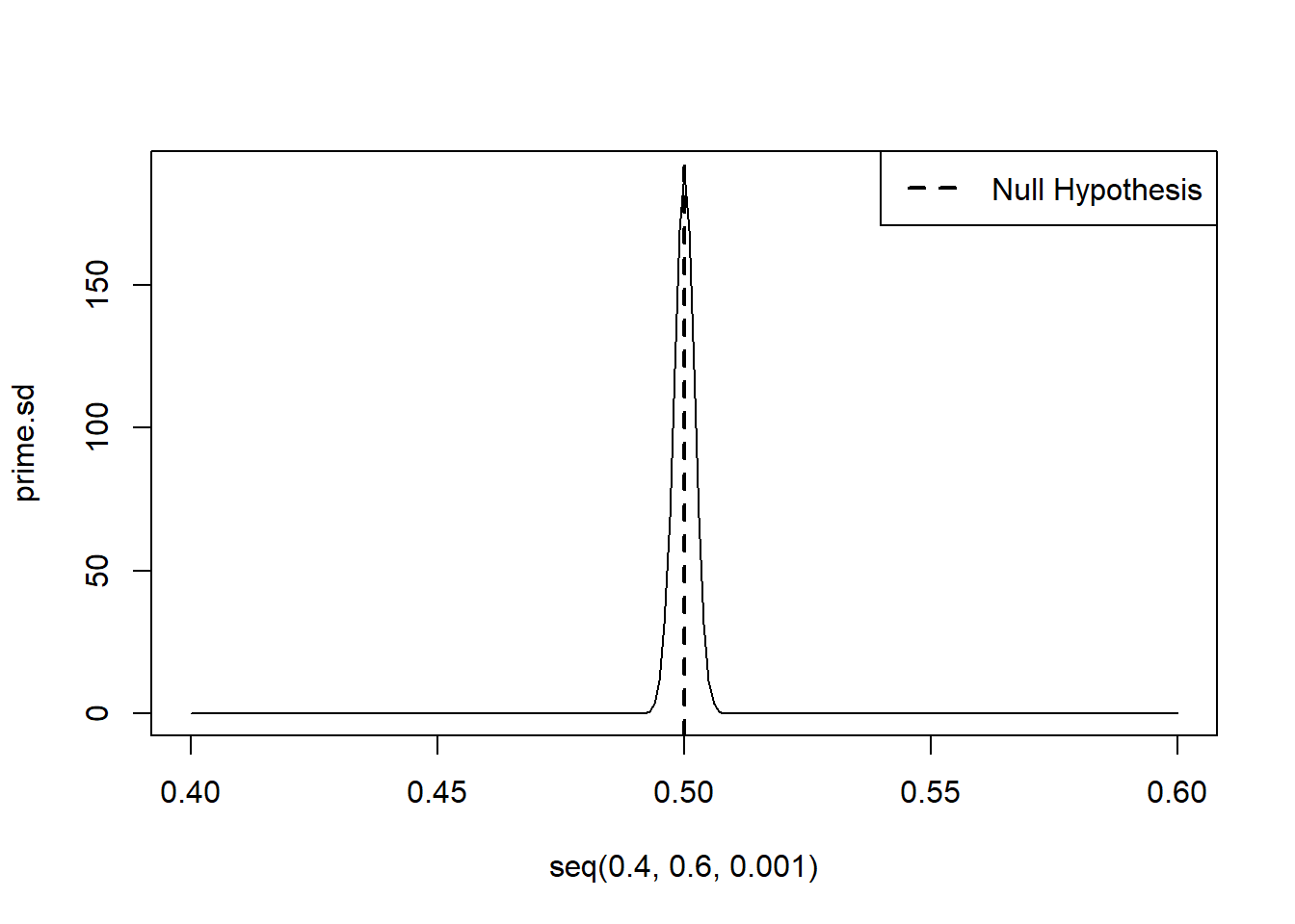
Again, this is our estimate of what sort of estimates would be produced if the null hypothesis was true. We would expect a lot of the estimate to be right around 50%. 51% and 49% are possible. 45% and 55% are highly unlikely.
Why is this distribution so much smaller than the sampling distribution we produced in the previous part of the chapter when we had a sample of 300? Thinking about the equation for the standard error, the critical thing is that we divide by the square root of the sample size. For a given amount of standard deviation in our variable increased sample size will decrease the standard error. Because we take the square root there are diminishing returns to this (going from 100 to 200 matters, going from 200 to 300 matters but less than going from 100 to 200 etc). But obviously going from 300 to 55 thousand is going to impact things! This also makes good intuitive sense: when we have a larger group of people the small random streaks of too many people who oppose/support Trump will even out and we are much more likely to get something close to the population number.
- Determine whether our particular result is unlikely or likely if the null were true given the sampling distribution.
We can look visually to see where our estimate is relative to the sampling distribution under the null hypothesis:
plot(seq(.4,.6,.001), prime.sd, type="l")
abline(v=.5,lty=2, lwd=2)
abline(v=mean(sm.dat$trump.approve,na.rm=T), lty=2)
legend("topright", c("Null Hypothesis","Sample Mean"), lty=c(2,2), lwd=c(2,1))
Quite obviously it is extraordinarily unlikely to get something as extreme as what we got if the null were true. In this case it is so unlikely that I would reject the null hypothesis as being plausible. Trump’s approval is not 50% in the population.
All of that visualization is for demonstration purposes, really we can get the answer (and this is what I expect you to do) via the t.test command.
t.test(sm.dat$trump.approve, mu=.5)
#>
#>  One Sample t-test
#>
#> data:  sm.dat$trump.approve
#> t = -44.269, df = 54313, p-value < 2.2e-16
#> alternative hypothesis: true mean is not equal to 0.5
#> 95 percent confidence interval:
#>  0.4025595 0.4108219
#> sample estimates:
#> mean of x
#> 0.4066907
So here the p-value – the probability of observing the mean that we have observed if the null is true – is very low, clost to zero. Critically though, the p-value is not zero and should never be rounded down to zero.
If we want to visualize the p-value it is the cumulative area under the curve to the left of .407 in the graph above. (Sort of, a complication to this in the next paragraph.) This is a very small amount of total probability, but because that line never actually touches zero the amount of area under that curve can never be exactly zero. So never round a p-value down to zero.
The other complication to this is that the standard hypothesis test we run is a “two-tailed” hypothesis. When we set up our hypothesis test we set the null hypothesis as being whether Trump’s approval is 50%, or not. Because we were ambivalent about whether we think it might be greater or lower than that number, we actually determine the probability of to the left of our value and to the right of the mean value flipped to the other side of the null hypothesis:
prime.sd <- dnorm(seq(.4,.6,.001), mean=.5, sd=se)
plot(seq(.4,.6,.001), prime.sd, type="l")
abline(v=.5,lty=2, lwd=2)
abline(v=mean(sm.dat$trump.approve,na.rm=T), lty=2)
abline(v= 1-mean(sm.dat$trump.approve,na.rm=T), lty=2)
legend("topright", c("Null Hypothesis","Sample Mean"), lty=c(2,2), lwd=c(2,1))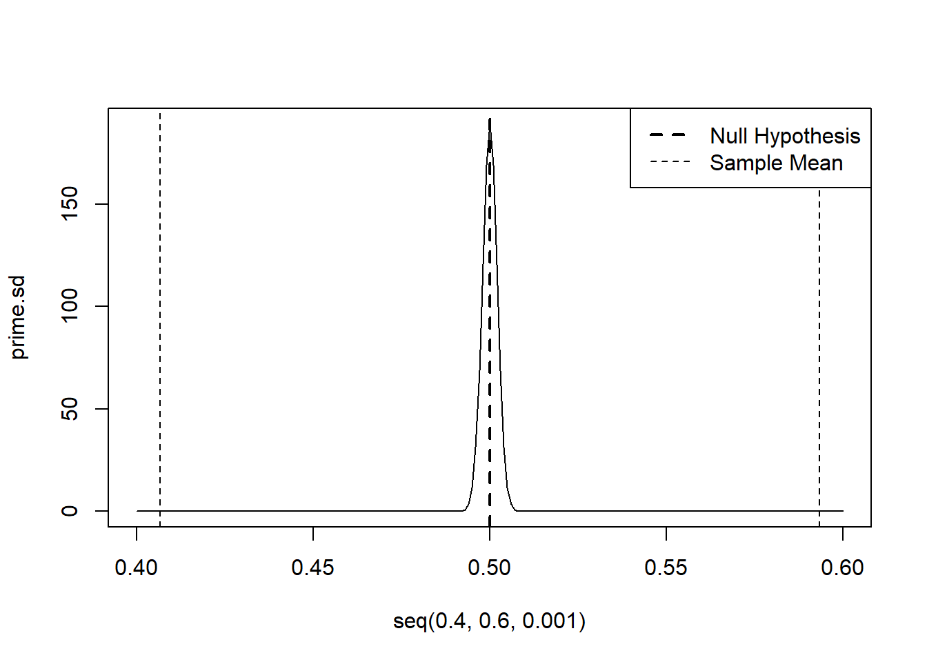
(If you don’t want to worry about this, then don’t. You can still just think about the p-value in the way I discussed above. )
Note, again, that the t.test function will automatically assume that the null is 0 if you don’t specify:
t.test(sm.dat$trump.approve)
#>
#>  One Sample t-test
#>
#> data:  sm.dat$trump.approve
#> t = 192.95, df = 54313, p-value < 2.2e-16
#> alternative hypothesis: true mean is not equal to 0
#> 95 percent confidence interval:
#>  0.4025595 0.4108219
#> sample estimates:
#> mean of x
#> 0.4066907
That’s not what we want in this case, so good to be careful!
Like everything, we can save the output of the t.test as an object and see some extra information
One note on confidence intervals: there real definition is somewhat confusing to the point that I generally recommend avoiding them until you have a firmer grasp on what it is that they are representing. The true definition of a confidence interval is that 95 out of 100 similarly constructed confidence intervals will contain the true population paramater. This is a big different then what people think so things can get confusing. I would stick to the relatively understandable definition of p-values I provided above.
10.4.1 Difference in means
What about a more complciated question using this data?
Data: Whether Americans approve (1) or not (0) of Donald Trump in September, with party
Question: Do Democrats and Republicans have different approval rates of the president?
Statistic: % Approve of Trump among Ds and Rs
Null Hypothesis: Democrats and Republicans have the same level of approval of Trump
% Approve_D == % Approve_R OR % Approve_D - % Approve_R==0.
Before we were looking at one mean and determining whether it was plausible against some null hypothesis. In this case we are looking at two means and determining whether they are different from one another.
head(sm.dat)
#>         trump.approve dem rep      party
#> 1207838             1   0   0       <NA>
#> 1223744             0   1   0   Democrat
#> 1229482             1   0   1 Republican
#> 1232667             0   1   0   Democrat
#> 1237784             0   1   0   Democrat
#> 1238590             1   0   1 Republican
mean(sm.dat$trump.approve[sm.dat$party=="Democrat"],na.rm=T)
#> [1] 0.0380243
mean(sm.dat$trump.approve[sm.dat$party=="Republican"],na.rm=T)
#> [1] 0.8872213
Just eyeballing this: yes these two values are different.
But if we are thinking in a “what is data” fashion we have the same sort of questions and concerns. Every time we get a new sample we are going to get slightly different values for the mean among democrats and the mean among republicans, and therefore, a different value for the difference in those two means. Given that underlying uncertainty what we can conclude about the plausability of what the true value is in the population.
Going through our 4 step process again:
- Calculate a statistic in our sample.
Here the statistic is the difference in the two means:
mean(sm.dat$trump.approve[sm.dat$party=="Democrat"],na.rm=T) - mean(sm.dat$trump.approve[sm.dat$party=="Republican"],na.rm=T)
#> [1] -0.849197- State the null hypothesis.
For a difference in means test we almost always have the same null hypothesis: that the difference is zero. This would indicate that the means are the same in the population.
- Estimate the distribution of the statistic if the null were true in an infinite number of samples. (The sampling distribution).
We know that the sampling distribution is centered on 0, but what is it’s shape? Again, we think that sampling distributions are normally distributed so really we just need to know the standard error. There is a way to calculate this, but from here on we are going to let the t.test function handle this for us, so we can combine this with….
- Determine whether our particular result is unlikely or likely if the null were true given the sampling distribution.
To do a difference in means test we can put both variables into the t.test function:
t.test(sm.dat$trump.approve[sm.dat$party=="Democrat"],sm.dat$trump.approve[sm.dat$party=="Republican"])
#>
#>  Welch Two Sample t-test
#>
#> data:  sm.dat$trump.approve[sm.dat$party == "Democrat"] and sm.dat$trump.approve[sm.dat$party == "Republican"]
#> t = -341, df = 33050, p-value < 2.2e-16
#> alternative hypothesis: true difference in means is not equal to 0
#> 95 percent confidence interval:
#>  -0.8540781 -0.8443159
#> sample estimates:
#> mean of x mean of y
#> 0.0380243 0.8872213
This gives us both means and that the alternative hypothesis is that the difference in means is not equal to 0. (In other words the null hypothesis is that the difference is equal to 0). We see a very low p-value, indicating that the there is a very low probability of observing a difference this large if the true difference was 0.
We can extract the standard error from this if we want. There is a way to calculate this standard error that’s slightly different from what’s above from a single mean. We aren’t going to discuss the equation here but it is very similar where the randomness of the variables in the dataset are divided by the group sizes.
se <- t.test(sm.dat$trump.approve[sm.dat$party=="Democrat"],sm.dat$trump.approve[sm.dat$party=="Republican"])$stderrAnd visualize the sampling distribution under the null hypothesis:
diff <- seq(-1,1,.001)
dens <- dnorm(diff, mean=0, sd=se)

plot(diff, dens, type="l", main="Null Sampling Distribution for Difference in Means")
abline(v=mean(sm.dat$trump.approve[sm.dat$party=="Democrat"],na.rm=T) - mean(sm.dat$trump.approve[sm.dat$party=="Republican"],na.rm=T))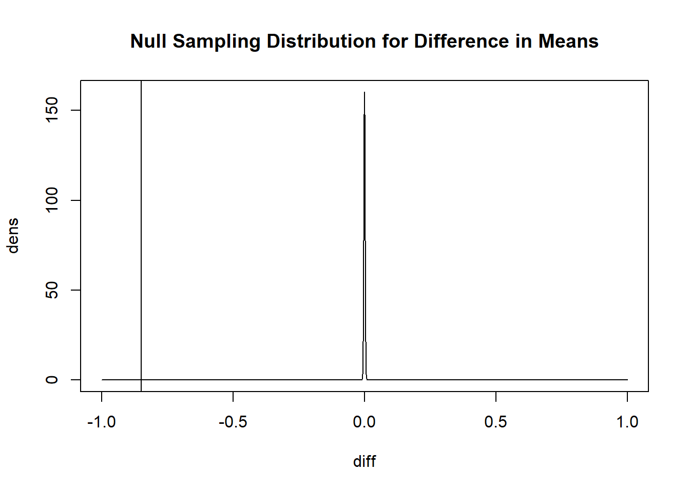
Again, you don’t need to make these visualizations. I’m just doing so to give you a better sense of what these hypothesis tests are saying. Here if the true difference in means was 0 we would be insanely unlikely to get this result in a sample. So we are very confident in rejecting the null hypothesis of no difference.
Note, also, that a difference in means test can be entered into the t.test function via a formula. If you have one variable that you want the mean of, and a second variable which has two values, you can use a tilde (~) and R will#do the rest!
t.test(sm.dat$trump.approve ~ sm.dat$party)
#>
#>  Welch Two Sample t-test
#>
#> data:  sm.dat$trump.approve by sm.dat$party
#> t = -341, df = 33050, p-value < 2.2e-16
#> alternative hypothesis: true difference in means between group Democrat and group Republican is not equal to 0
#> 95 percent confidence interval:
#>  -0.8540781 -0.8443159
#> sample estimates:
#>   mean in group Democrat mean in group Republican
#>                0.0380243                0.8872213
Let’s load in the ACS data to get a couple more examples:
acs <- rio::import("https://github.com/marctrussler/IDS-Data/raw/main/ACSCountyData.csv")One of the variables in the dataset is the percent of people who commute by car in each county. What if I want to test the null hypothesis that the average percent commuting by car is 100%?
mean(acs$percent.car.commute, na.rm=T)
#> [1] 89.36677
We see that the mean here is 89%
Remember, even though this feels like the truth – this is the census bureau afterall – this is still a sample and this is still an estimate. It’s possible, if we ran the ACS again and again, the underlying randomness might produce a number like 89% even if the truth was 100%. We can test this in the same way, but changing mu to be our null of 100:
t.test(acs$percent.car.commute, mu=100)
#>
#>  One Sample t-test
#>
#> data:  acs$percent.car.commute
#> t = -79.835, df = 3140, p-value < 2.2e-16
#> alternative hypothesis: true mean is not equal to 100
#> 95 percent confidence interval:
#>  89.10562 89.62792
#> sample estimates:
#> mean of x
#>  89.36677
We see after our test that it’s very unlikely to get something this extreme if the truth was 100%.
What about if we wanted to know if the percent car commuting is different in the south or not the south?
We have region, but that has too many categories:
#Won't work:
#t.test(acs$percent.car.commute ~ acs$census.region)
Let’s create a variable for south
acs$south <- NA
acs$south[acs$census.region=="south"] <- 1
acs$south[acs$census.region!="south"] <- 0
Now we can run a t.test
t.test(acs$percent.car.commute ~ acs$south)
#>
#>  Welch Two Sample t-test
#>
#> data:  acs$percent.car.commute by acs$south
#> t = -22.754, df = 2584.1, p-value < 2.2e-16
#> alternative hypothesis: true difference in means between group 0 and group 1 is not equal to 0
#> 95 percent confidence interval:
#>  -5.825462 -4.901063
#> sample estimates:
#> mean in group 0 mean in group 1
#>        86.93871        92.30197
All of these t-tests have been pretty obvious thus far, but that’s not always going to be the case. There are lots of times where an apparent difference in means (or regression coefficient) are not statistically significant: there is not enough evidence to overturn the idea that we could see something as extreme just due to the underlying randomness inherent in taking samples. But the basic logic is the same, and it’s something you should ALWAYS be thinking about.
The point of statistics is not to describe the data we have, but the population which we can’t observe. We can think about our data, and any estimate we calculate in our data, as one of an infinite number of possibilities, all a bit different. Thankfully, we are really good at estimating what the distribution of all these possibilities are (a sampling distribution), and from that can calculate how likely our estimated value is assuming that the null hypothesis was true.