4 Data Frames
Thus far we have been working with vectors and matrices of data using Rs square-bracket-coordinate system: referring to different columns, rows, or individual numbers based on their index numbers.
This all seems a bit hard. When we work with data in R are we really going to have to remember which column is all the time? What if income is the third column but then we add data columns to the start and income becomes the sixth column? That would be terrible.
I started with thinking about R using the square brackets and index positions because it is, in some sense, the “grammar” of R. Thinking about everything as a vector or matrix with index positions is really how R thinks about storing and accesing data. Being conversant in that grammar will make you a more flexible coder in the future.
But to make things easier we are going to use a special object in R designed to make traditional analysis easier, the dataframe.
The first dataframe we are going to make use of is data from the American Community Survey (ACS) on features of all the counties in the United States.
I would like to, again, think about how we can load data in when that data is downloaded to our computers. The file ACSCountyData.Rds is available to download on canvas.
Now I downloaded the file into the folder on my computer for this class in a sub-folder called “Data”. I’m going to use the file explorer on my computer to navigate to that file on my computer.
Because I’m using a windows computer I’m going to hold down the shift key and then right click the file. When I do this the option “Copy as path” will appear in the menu. I’m going to click that button. We can now paste that filepath into the same import command that we used to load data from a github url. One last complication on a Windows computer is that the “copy as path” trick gives a filepath with the slashes going in the wrong direction. You just have to change the \ to /, which you can do manually or via find-and-replace (ctrl-f).
If you are using an Apple computer (and most of you are) you are also going to navigate to the downloaded file using finder. Right click (control + click, or two finger click on trackpad) on the file and a context menu with options will popup. Hold the option key then the options will change and you would be able to see the option: Copy "folder_name" as Pathname. Click on it, the full path of the file/folder would be copied to the clipboard. You can now paste the full path into the import command. You do not have to change the direction of the slashes.
library(rio)
#You will have to paste your own filepath into the import command
#Notice that the ACS data is a different file type (CSV), but the import command works just fine to figure it out.
acs <- import("C:/Users/trussler-adm/PORES Dropbox/PORES/PSCI1800/Data/ACSCountyData.csv")
A helpful shortcut to loading in data is to set the “working directory” for an R session. I can tell R that a particular folder is the one i’m working out of for a project. The ACS data is also the data I use in the example problem set folder. I can load that in using the method we have already set out:
#Same data in a different location on my computer
acs <- import("C:/Users/trussler-adm/PORES Dropbox/PORES/PSCI1800/Problem Sets/Example Problem Set Folder/Data/ACSCountyData.Rdata")
But in a big project (like your final projects) I may have many different data sources all located in the same place. I can, helpfully, tell R that this is the project folder.
setwd("C:/Users/trussler-adm/PORES Dropbox/PORES/PSCI1800/Problem Sets/Example Problem Set Folder")
#Check to see if that worked
getwd()
#> [1] "C:/Users/trussler-adm/PORES Dropbox/PORES/PSCI1800/Problem Sets/Example Problem Set Folder"
After doing that, I can load the data relative to the working directory:
setwd("C:/Users/trussler-adm/PORES Dropbox/PORES/PSCI1800/Problem Sets/Example Problem Set Folder")
acs <- import("Data/ACSCountyData.Rdata")
This might seem pedantic and a bit over-complicated, but things like this become much more helpful when you are working on “real” data science projects. On the papers I write for publication I might be working with 10 or 20 raw data files and might be producing 50 to 100 figures. It would be too complicated to have everything all mushed together in one big folder (or all in my downloads folder, which is a big no-no). Again: understanding how this system works is also just a prerequisite to being taken seriously as a data scientist in the real world.
One caveat to the working directory thing is that it works a little different for an Rmarkdown file, which you will be using for your problem sets and final projects. For an Rmarkdown file the working directory is automatically set to wherever you have your .Rmd file saved.
#Backup link to load acs data from the github:
acs <- import("https://github.com/marctrussler/IDS-Data/raw/main/ACSCountyData.csv")
Now we can start working with acs we can see that it is loaded into the environment and has a special little blue arrow beside it, which tells us that this is a data frame. We can confirm with:
class(acs)
#> [1] "data.frame"
We can click on the object and it will open in a new window for us to look at it. We can also use the View() command:
#View is one of the very few capitalized commands. How did this happen? Why did they do this? What is anything?
#View(acs)
Last week we dipped our toes into data frames because one of their key features is that we can combine different classes of data into one matrix. We can see that acs has a combination of character (words) and numeric data.
In the View() display we cannot click and edit any of the data, but it should be clear about what that is. Doing so would go directly against what we have learned about good coding practice.
Whenever I open a new dataset the first thing I think about is the unit of analysis. This is a fancy way of saying: what does each row uniquely represent? In some cases this is very obvious. For acs the unit of analysis is a county. Each row in the dataset is a county, and there are no repeated counties.
But consider this dataset:
pres <- import("https://github.com/marctrussler/IDS-Data/raw/main/PresElection.Rds")
#View(pres)
On first blush it looks like the unit of analysis of this dataset is also county. But note above that I said: what does each row uniquely represent. What happens if I click on the county.fips row to sort it by census generated fips codes? We see that county 1001 (which is Autugua county, Alabama) is in the data 6 times. So it’s not the case that county uniquely identifies rows. Instead, each row represents a “county-year”.
Here are some other basic tools for understanding a dataset.
Each column in a dataset is named, and we can get a vector of those names:
names(acs)
#>  [1] "V1"                      "county.fips"
#>  [3] "county.name"             "state.full"
#>  [5] "state.abbr"              "state.alpha"
#>  [7] "state.icpsr"             "census.region"
#>  [9] "population"              "population.density"
#> [11] "percent.senior"          "percent.white"
#> [13] "percent.black"           "percent.asian"
#> [15] "percent.amerindian"      "percent.less.hs"
#> [17] "percent.college"         "unemployment.rate"
#> [19] "median.income"           "gini"
#> [21] "median.rent"             "percent.child.poverty"
#> [23] "percent.adult.poverty"   "percent.car.commute"
#> [25] "percent.transit.commute" "percent.bicycle.commute"
#> [27] "percent.walk.commute"    "average.commute.time"
#> [29] "percent.no.insurance"
If we want to look at the first 6 rows of the data for all variables:
head(acs)
#>   V1 county.fips     county.name state.full state.abbr
#> 1  1        1055   Etowah County    Alabama         AL
#> 2  2        1133  Winston County    Alabama         AL
#> 3  3        1053 Escambia County    Alabama         AL
#> 4  4        1001  Autauga County    Alabama         AL
#> 5  5        1003  Baldwin County    Alabama         AL
#> 6  6        1005  Barbour County    Alabama         AL
#>   state.alpha state.icpsr census.region population
#> 1           1          41         south     102939
#> 2           1          41         south      23875
#> 3           1          41         south      37328
#> 4           1          41         south      55200
#> 5           1          41         south     208107
#> 6           1          41         south      25782
#>   population.density percent.senior percent.white
#> 1          192.30800       18.33804      80.34856
#> 2           38.94912       21.05550      96.33927
#> 3           39.49123       17.34891      61.87045
#> 4           92.85992       14.58333      76.87862
#> 5          130.90190       19.54043      86.26620
#> 6           29.13214       17.97378      47.38189
#>   percent.black percent.asian percent.amerindian
#> 1    15.7491330     0.7179009          0.7295583
#> 2     0.3769634     0.1298429          0.3895288
#> 3    31.9331333     0.3616588          3.8496571
#> 4    19.1394928     1.0289855          0.2880435
#> 5     9.4970376     0.8072770          0.7313545
#> 6    47.5758281     0.3723528          0.2792646
#>   percent.less.hs percent.college unemployment.rate
#> 1       15.483020        17.73318          6.499382
#> 2       21.851723        13.53585          7.597536
#> 3       18.455613        12.65935         13.461675
#> 4       11.311414        27.68929          4.228036
#> 5        9.735422        31.34588          4.444240
#> 6       26.968580        12.21592          9.524798
#>   median.income   gini median.rent percent.child.poverty
#> 1         44023 0.4483         669              30.00183
#> 2         38504 0.4517         525              23.91744
#> 3         35000 0.4823         587              33.89582
#> 4         58786 0.4602         966              22.71976
#> 5         55962 0.4609         958              13.38019
#> 6         34186 0.4731         590              47.59704
#>   percent.adult.poverty percent.car.commute
#> 1              15.42045            94.28592
#> 2              15.83042            94.63996
#> 3              23.50816            98.54988
#> 4              14.03953            95.15310
#> 5              10.37312            91.71079
#> 6              25.40757            94.22581
#>   percent.transit.commute percent.bicycle.commute
#> 1              0.20813669              0.08470679
#> 2              0.38203288              0.00000000
#> 3              0.00000000              0.06667222
#> 4              0.10643524              0.05731128
#> 5              0.08969591              0.05797419
#> 6              0.25767159              0.00000000
#>   percent.walk.commute average.commute.time
#> 1            0.8373872                   24
#> 2            0.3473026                   29
#> 3            0.4250354                   23
#> 4            0.6263304                   26
#> 5            0.6956902                   27
#> 6            2.1316468                   23
#>   percent.no.insurance
#> 1            10.357590
#> 2            12.150785
#> 3            14.308294
#> 4             7.019928
#> 5            10.025612
#> 6             9.921651
… or the last 6 rows:
tail(acs)
#>        V1 county.fips       county.name state.full
#> 3137 3137       56031     Platte County    Wyoming
#> 3138 3138       56033   Sheridan County    Wyoming
#> 3139 3139       56035   Sublette County    Wyoming
#> 3140 3140       56037 Sweetwater County    Wyoming
#> 3141 3141       56039      Teton County    Wyoming
#> 3142 3142       56041      Uinta County    Wyoming
#>      state.abbr state.alpha state.icpsr census.region
#> 3137         WY          50          68          west
#> 3138         WY          50          68          west
#> 3139         WY          50          68          west
#> 3140         WY          50          68          west
#> 3141         WY          50          68          west
#> 3142         WY          50          68          west
#>      population population.density percent.senior
#> 3137       8673           4.166810       23.44056
#> 3138      30012          11.893660       19.63881
#> 3139       9951           2.036434       16.72194
#> 3140      44117           4.231043       10.70109
#> 3141      23059           5.769299       13.59556
#> 3142      20609           9.899982       12.12092
#>      percent.white percent.black percent.asian
#> 3137      94.81148    0.01153004     0.6802721
#> 3138      95.07530    0.50979608     0.7030521
#> 3139      96.25163    0.00000000     0.1205909
#> 3140      93.12510    0.80241177     0.6324093
#> 3141      90.34217    1.18825621     1.2229498
#> 3142      93.41550    0.09704498     0.1067495
#>      percent.amerindian percent.less.hs percent.college
#> 3137         0.08071025        6.589393        21.73706
#> 3138         1.22617620        4.801207        29.98632
#> 3139         0.43211738        3.676471        25.24510
#> 3140         1.68189133        8.996576        22.03438
#> 3141         0.33392602        5.581450        57.37008
#> 3142         0.77635984        7.231901        15.44715
#>      unemployment.rate median.income   gini median.rent
#> 3137          2.666667         47096 0.4635         746
#> 3138          2.685430         58521 0.4383         809
#> 3139          3.409091         78680 0.3580         980
#> 3140          5.196641         73008 0.4127         868
#> 3141          1.445584         83831 0.4879        1339
#> 3142          6.054630         58235 0.4002         664
#>      percent.child.poverty percent.adult.poverty
#> 3137             20.304569             10.058188
#> 3138              6.346244              6.317891
#> 3139             10.041667              8.343327
#> 3140             14.092187             11.206294
#> 3141              4.212911              8.344662
#> 3142             15.980066             11.091579
#>      percent.car.commute percent.transit.commute
#> 3137            85.61220               0.6193425
#> 3138            87.57592               0.1214739
#> 3139            86.50675               0.3373313
#> 3140            89.88532               2.7568807
#> 3141            72.18383               4.0541503
#> 3142            92.80077               3.6049488
#>      percent.bicycle.commute percent.walk.commute
#> 3137               0.8575512            4.1686517
#> 3138               0.4251586            2.7534080
#> 3139               0.5997001            4.9100450
#> 3140               0.2522936            3.5045872
#> 3141               3.0495191           12.8678304
#> 3142               0.3306314            0.8532423
#>      average.commute.time percent.no.insurance
#> 3137                   17             9.927361
#> 3138                   16             9.542850
#> 3139                   20            13.365491
#> 3140                   20            11.877508
#> 3141                   15             9.996097
#> 3142                   21            12.125770
To get some basic summary statistics for all variable:
summary(acs)
#>        V1          county.fips    county.name
#>  Min.   :   1.0   Min.   : 1001   Length:3142
#>  1st Qu.: 786.2   1st Qu.:18178   Class :character
#>  Median :1571.5   Median :29176   Mode  :character
#>  Mean   :1571.5   Mean   :30384
#>  3rd Qu.:2356.8   3rd Qu.:45081
#>  Max.   :3142.0   Max.   :56045
#>
#>   state.full         state.abbr         state.alpha
#>  Length:3142        Length:3142        Min.   : 1.00
#>  Class :character   Class :character   1st Qu.:14.00
#>  Mode  :character   Mode  :character   Median :25.00
#>                                        Mean   :26.34
#>                                        3rd Qu.:40.00
#>                                        Max.   :50.00
#>                                        NA's   :1
#>   state.icpsr    census.region        population
#>  Min.   : 1.00   Length:3142        Min.   :      75
#>  1st Qu.:32.00   Class :character   1st Qu.:   10948
#>  Median :43.00   Mode  :character   Median :   25736
#>  Mean   :41.45                      Mean   :  102770
#>  3rd Qu.:51.00                      3rd Qu.:   67209
#>  Max.   :82.00                      Max.   :10098052
#>
#>  population.density percent.senior   percent.white
#>  Min.   :    0.04   Min.   : 3.799   Min.   :  3.891
#>  1st Qu.:   16.69   1st Qu.:15.448   1st Qu.: 76.631
#>  Median :   44.72   Median :18.038   Median : 89.636
#>  Mean   :  270.68   Mean   :18.364   Mean   : 83.055
#>  3rd Qu.:  116.71   3rd Qu.:20.805   3rd Qu.: 95.065
#>  Max.   :72052.96   Max.   :55.596   Max.   :100.000
#>
#>  percent.black     percent.asian    percent.amerindian
#>  Min.   : 0.0000   Min.   : 0.000   Min.   : 0.0000
#>  1st Qu.: 0.6738   1st Qu.: 0.291   1st Qu.: 0.1712
#>  Median : 2.2673   Median : 0.606   Median : 0.3498
#>  Mean   : 9.0596   Mean   : 1.373   Mean   : 1.9671
#>  3rd Qu.:10.1602   3rd Qu.: 1.315   3rd Qu.: 0.8419
#>  Max.   :87.4123   Max.   :42.511   Max.   :92.4799
#>
#>  percent.less.hs  percent.college unemployment.rate
#>  Min.   : 1.183   Min.   : 0.00   Min.   : 0.000
#>  1st Qu.: 8.755   1st Qu.:15.00   1st Qu.: 3.982
#>  Median :12.081   Median :19.25   Median : 5.447
#>  Mean   :13.409   Mean   :21.57   Mean   : 5.774
#>  3rd Qu.:17.184   3rd Qu.:25.57   3rd Qu.: 7.073
#>  Max.   :66.344   Max.   :78.53   Max.   :28.907
#>                                   NA's   :1
#>  median.income         gini         median.rent
#>  Min.   : 20188   Min.   :0.2567   Min.   : 318
#>  1st Qu.: 42480   1st Qu.:0.4210   1st Qu.: 622
#>  Median : 49888   Median :0.4432   Median : 700
#>  Mean   : 51583   Mean   :0.4454   Mean   : 757
#>  3rd Qu.: 57611   3rd Qu.:0.4673   3rd Qu.: 829
#>  Max.   :136268   Max.   :0.6647   Max.   :2158
#>  NA's   :1        NA's   :1        NA's   :3
#>  percent.child.poverty percent.adult.poverty
#>  Min.   : 0.00         Min.   : 0.00
#>  1st Qu.:14.26         1st Qu.:10.42
#>  Median :20.32         Median :14.18
#>  Mean   :21.49         Mean   :15.05
#>  3rd Qu.:26.90         3rd Qu.:18.44
#>  Max.   :72.59         Max.   :52.49
#>  NA's   :2             NA's   :1
#>  percent.car.commute percent.transit.commute
#>  Min.   : 7.947      Min.   : 0.0000
#>  1st Qu.:87.726      1st Qu.: 0.1081
#>  Median :91.161      Median : 0.3639
#>  Mean   :89.367      Mean   : 0.9812
#>  3rd Qu.:93.448      3rd Qu.: 0.8106
#>  Max.   :99.084      Max.   :61.9243
#>  NA's   :1           NA's   :1
#>  percent.bicycle.commute percent.walk.commute
#>  Min.   : 0.0000         Min.   : 0.000
#>  1st Qu.: 0.0000         1st Qu.: 1.333
#>  Median : 0.1405         Median : 2.240
#>  Mean   : 0.3308         Mean   : 3.175
#>  3rd Qu.: 0.3842         3rd Qu.: 3.734
#>  Max.   :10.9091         Max.   :53.784
#>  NA's   :1               NA's   :1
#>  average.commute.time percent.no.insurance
#>  Min.   : 5.00        Min.   : 1.524
#>  1st Qu.:20.00        1st Qu.: 6.060
#>  Median :23.00        Median : 8.933
#>  Mean   :23.57        Mean   : 9.811
#>  3rd Qu.:27.00        3rd Qu.:12.334
#>  Max.   :45.00        Max.   :45.518
#>  NA's   :2
We also might want to understand the dimensions of our dataset. Now I can look over to the environment and see that there are 3220 observations (rows) and 28 variables (columns), but in the future we may want to actually produce those numbers and use them in functions. We can do so with:
The key feature of a data frame which makes them much easier to use compared to the simple matrices we have been using up to this point is that we can refer to columns by their name using $.
If we want to look at the population of all the counties, before we would use the fact that it is the 8th column and type:
head(acs[,8])
#> [1] "south" "south" "south" "south" "south" "south"
But now we can use the name. Note that when I type the dollar sign R will pop open all the names for me:
head(acs$population)
#> [1] 102939  23875  37328  55200 208107  25782
Because population is a vector of information I can still use the square brackets to index it and pull out specific values:
acs$population[2:4]
#> [1] 23875 37328 55200
And I can easily run the same sort of statistics on this named variable as I did when we were referring to variables by number:
mean(acs$population)
#> [1] 102769.9

max(acs$population)
#> [1] 10098052

median(acs$population)
#> [1] 25736
We are also able to perform arithmetic on these variables the same as we have been doing before. For example, if I want to have a variable that is population in thousands I can do:
head(acs$population/1000)
#> [1] 102.939  23.875  37.328  55.200 208.107  25.782
I can save this as an object:
pop.1000 <- acs$population/1000But that doesn’t really make any sense, why am I saving something that is the same length as acs as a seperate variable? I want this to be a new column in the dataset. To do so all I need to do is use the assignment operator:
acs$pop.1000 <- acs$population/1000We can see that acs now has 29 columns, because we added a new variable:
ncol(acs)
#> [1] 30
If we want a variable that is the percent of the county that is neither white or black:
acs$perc.non.white.black <- 100 - (acs$percent.white + acs$percent.black)
head(acs$perc.non.white.black)
#> [1] 3.902311 3.283770 6.196421 3.981884 4.236763 5.042278
For a dataset this long, we might be interested in quickly figuring out what all of the possible values are. We can do that with unique().
unique(acs$census.region)
#> [1] "south"     "west"      "northeast" "midwest"
If we also want to determine how frequently the different options show up, we can use the table command:
table(acs$census.region)
#>
#>   midwest northeast     south      west
#>      1055       217      1422       448
This is telling us how many rows that variable takes on each value. In real terms, this is how many counties are in each region.
If you would like proportions instead of counts, you can wrap that whole command in prop.table():
prop.table(table(acs$census.region))
#>
#>    midwest  northeast      south       west
#> 0.33577339 0.06906429 0.45257798 0.14258434
You have to be a little bit smart when using these commands. If I apply the table command to a continuous variable i’m just going to get nonsense back:
#Uncomment and run
#table(acs$population)
A final important command is the order function. For a given variable, this function will return the row numbers sorted from smallest to largest
So row 551 contains the observation with the lowest population
acs[551,]
#>      V1 county.fips    county.name state.full state.abbr
#> 551 551       15005 Kalawao County     Hawaii         HI
#>     state.alpha state.icpsr census.region population
#> 551          11          82          west         75
#>     population.density percent.senior percent.white
#> 551           6.254478             16      21.33333
#>     percent.black percent.asian percent.amerindian
#> 551      2.666667            28           2.666667
#>     percent.less.hs percent.college unemployment.rate
#> 551        13.04348        24.63768                 0
#>     median.income   gini median.rent percent.child.poverty
#> 551         61875 0.3589         863                    NA
#>     percent.adult.poverty percent.car.commute
#> 551              11.86441            43.63636
#>     percent.transit.commute percent.bicycle.commute
#> 551                       0                10.90909
#>     percent.walk.commute average.commute.time
#> 551                   40                    5
#>     percent.no.insurance pop.1000 perc.non.white.black
#> 551             2.666667    0.075                   76
How can we see the end of this vector, which will tell us the row with the largest population?
We can use head() inverse, which (Accordingly) is tail()
This gives us the last 6 values of that vector
So what is the largest county?
acs[207,]
#>      V1 county.fips        county.name state.full
#> 207 207        6037 Los Angeles County California
#>     state.abbr state.alpha state.icpsr census.region
#> 207         CA           5          71          west
#>     population population.density percent.senior
#> 207   10098052           2488.312       12.86661
#>     percent.white percent.black percent.asian
#> 207      51.36495      8.159861      14.55695
#>     percent.amerindian percent.less.hs percent.college
#> 207          0.6984218         21.3384        31.80899
#>     unemployment.rate median.income   gini median.rent
#> 207          6.833541         64251 0.5022        1390
#>     percent.child.poverty percent.adult.poverty
#> 207              22.47003              14.28525
#>     percent.car.commute percent.transit.commute
#> 207             83.4639                6.210588
#>     percent.bicycle.commute percent.walk.commute
#> 207               0.8323332             2.716764
#>     average.commute.time percent.no.insurance pop.1000
#> 207                   31             10.76106 10098.05
#>     perc.non.white.black
#> 207             40.47519
And we see that, reasonably, LA County is the largest county with over 10 million people.
Another (slightly shorter) way to determine which rows match some logical condition is to use the which() command, which takes as it’s first argument a logical statement, and then returns the rows for which it is true:
For example, where are the places where median income is at its max and min?
which(acs$median.income==max(acs$median.income,na.rm=T))
#> [1] 2835
acs[2835,]
#>        V1 county.fips    county.name state.full state.abbr
#> 2835 2835       51107 Loudoun County   Virginia         VA
#>      state.alpha state.icpsr census.region population
#> 2835          46          40         south     385143
#>      population.density percent.senior percent.white
#> 2835           746.7396       8.637052      66.15387
#>      percent.black percent.asian percent.amerindian
#> 2835      7.460865      17.97306          0.2586052
#>      percent.less.hs percent.college unemployment.rate
#> 2835        6.486335        60.79087          3.489436
#>      median.income   gini median.rent percent.child.poverty
#> 2835        136268 0.3859        1813              3.771955
#>      percent.adult.poverty percent.car.commute
#> 2835              3.505573            85.70692
#>      percent.transit.commute percent.bicycle.commute
#> 2835                4.165227                0.191762
#>      percent.walk.commute average.commute.time
#> 2835             1.733159                   34
#>      percent.no.insurance pop.1000 perc.non.white.black
#> 2835             6.161608  385.143             26.38526

which(acs$median.income==min(acs$median.income,na.rm=T))
#> [1] 1435
acs[1435,]
#>        V1 county.fips      county.name  state.full
#> 1435 1435       28063 Jefferson County Mississippi
#>      state.abbr state.alpha state.icpsr census.region
#> 1435         MS          24          46         south
#>      population population.density percent.senior
#> 1435       7346           14.12874       14.90607
#>      percent.white percent.black percent.asian
#> 1435      13.32698      85.89709     0.4492241
#>      percent.amerindian percent.less.hs percent.college
#> 1435          0.1497414        25.18977          15.002
#>      unemployment.rate median.income   gini median.rent
#> 1435          7.535944         20188 0.4982         423
#>      percent.child.poverty percent.adult.poverty
#> 1435              65.40284               46.8599
#>      percent.car.commute percent.transit.commute
#> 1435            95.28509                       0
#>      percent.bicycle.commute percent.walk.commute
#> 1435                       0              1.91886
#>      average.commute.time percent.no.insurance pop.1000
#> 1435                   24             15.80452    7.346
#>      perc.non.white.black
#> 1435            0.7759325

which(acs$median.income==median(acs$median.income,na.rm=T))
#> [1] 1077
acs[1077,]
#>        V1 county.fips    county.name state.full state.abbr
#> 1077 1077       21079 Garrard County   Kentucky         KY
#>      state.alpha state.icpsr census.region population
#> 1077          17          51         south      17328
#>      population.density percent.senior percent.white
#> 1077           75.30685       17.44575      96.12188
#>      percent.black percent.asian percent.amerindian
#> 1077      1.108033     0.1385042          0.4039705
#>      percent.less.hs percent.college unemployment.rate
#> 1077        20.09433        16.79271          5.989682
#>      median.income   gini median.rent percent.child.poverty
#> 1077         49888 0.4325         689               25.1379
#>      percent.adult.poverty percent.car.commute
#> 1077              15.12774            92.42466
#>      percent.transit.commute percent.bicycle.commute
#> 1077               0.1780822                       0
#>      percent.walk.commute average.commute.time
#> 1077            0.3972603                   34
#>      percent.no.insurance pop.1000 perc.non.white.black
#> 1077             7.450369   17.328             2.770083
How does making a scatterplot work with dataframes? It’s exactly the same as what we have been doing, but we can now use names instead of column numbers.
plot(acs$median.income, acs$percent.child.poverty)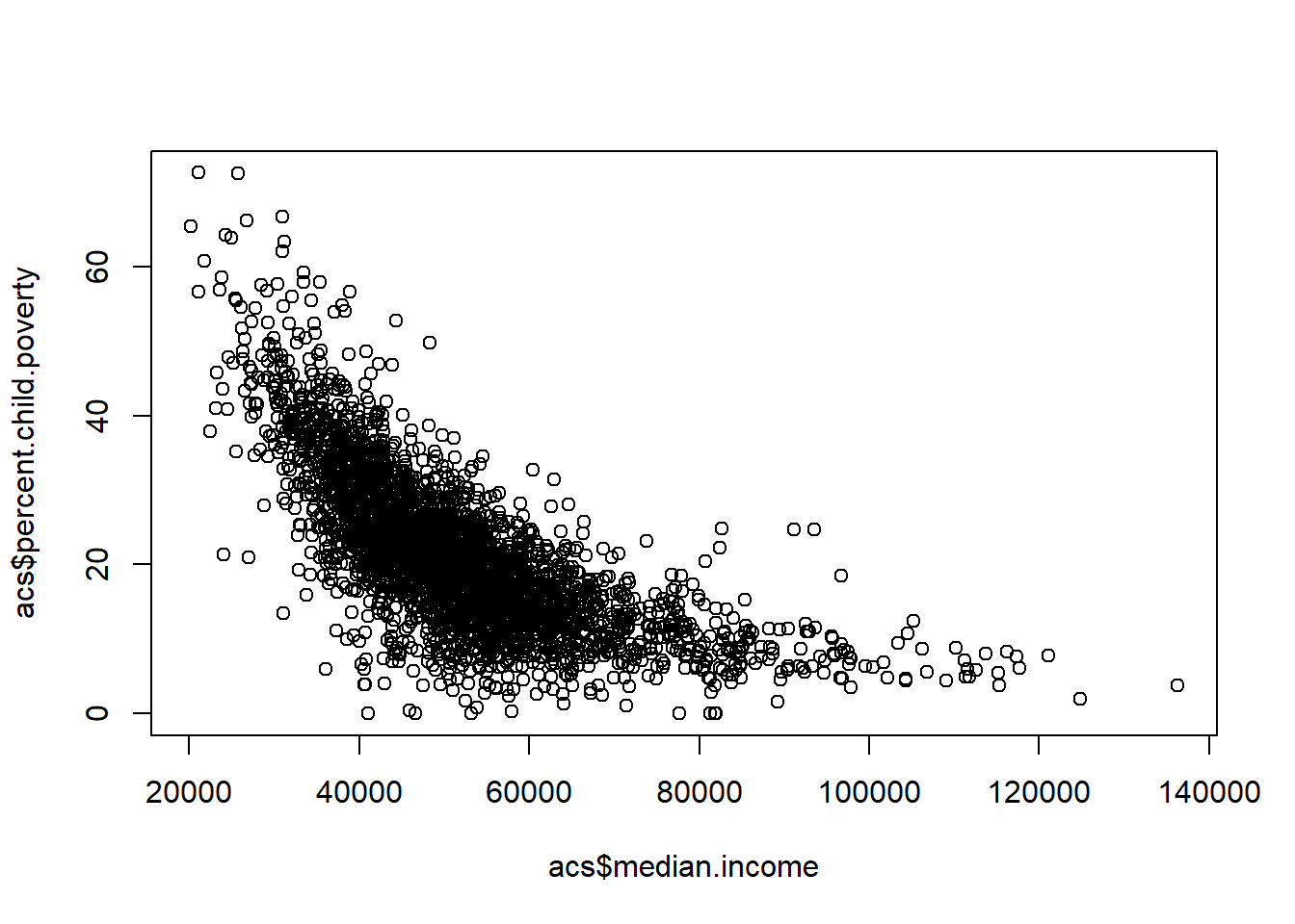
For the rest of the class – or if you are reading, for the next 10 minutes – work on making your own scatterplot using the ACS data to uncover a new relationship
4.1 Extending our knowledge of square brackets to dataframes
We’ve worked a lot to learn how to use square brackets in simple matrices, How can we extend this logic to working with a dataset?
For example: What are the first 10 rows in ACS?
acs[1:10,]
#>    V1 county.fips     county.name state.full state.abbr
#> 1   1        1055   Etowah County    Alabama         AL
#> 2   2        1133  Winston County    Alabama         AL
#> 3   3        1053 Escambia County    Alabama         AL
#> 4   4        1001  Autauga County    Alabama         AL
#> 5   5        1003  Baldwin County    Alabama         AL
#> 6   6        1005  Barbour County    Alabama         AL
#> 7   7        1007     Bibb County    Alabama         AL
#> 8   8        1009   Blount County    Alabama         AL
#> 9   9        1011  Bullock County    Alabama         AL
#> 10 10        1013   Butler County    Alabama         AL
#>    state.alpha state.icpsr census.region population
#> 1            1          41         south     102939
#> 2            1          41         south      23875
#> 3            1          41         south      37328
#> 4            1          41         south      55200
#> 5            1          41         south     208107
#> 6            1          41         south      25782
#> 7            1          41         south      22527
#> 8            1          41         south      57645
#> 9            1          41         south      10352
#> 10           1          41         south      20025
#>    population.density percent.senior percent.white
#> 1           192.30800       18.33804      80.34856
#> 2            38.94912       21.05550      96.33927
#> 3            39.49123       17.34891      61.87045
#> 4            92.85992       14.58333      76.87862
#> 5           130.90190       19.54043      86.26620
#> 6            29.13214       17.97378      47.38189
#> 7            36.19020       16.25161      76.65468
#> 8            89.39555       17.75176      95.50525
#> 9            16.62156       15.61051      21.98609
#> 10           25.77756       19.00624      52.00499
#>    percent.black percent.asian percent.amerindian
#> 1     15.7491330     0.7179009        0.729558282
#> 2      0.3769634     0.1298429        0.389528796
#> 3     31.9331333     0.3616588        3.849657094
#> 4     19.1394928     1.0289855        0.288043478
#> 5      9.4970376     0.8072770        0.731354544
#> 6     47.5758281     0.3723528        0.279264603
#> 7     22.2754916     0.1642473        0.035512940
#> 8      1.4953595     0.3434817        0.244600572
#> 9     76.2461360     0.5409583        1.178516229
#> 10    45.2184769     1.1535581        0.009987516
#>    percent.less.hs percent.college unemployment.rate
#> 1        15.483020        17.73318          6.499382
#> 2        21.851723        13.53585          7.597536
#> 3        18.455613        12.65935         13.461675
#> 4        11.311414        27.68929          4.228036
#> 5         9.735422        31.34588          4.444240
#> 6        26.968580        12.21592          9.524798
#> 7        16.793409        11.48923          7.513989
#> 8        19.837485        12.64289          4.084475
#> 9        24.774775        13.30236         11.060948
#> 10       15.416187        16.09303          6.708471
#>    median.income   gini median.rent percent.child.poverty
#> 1          44023 0.4483         669              30.00183
#> 2          38504 0.4517         525              23.91744
#> 3          35000 0.4823         587              33.89582
#> 4          58786 0.4602         966              22.71976
#> 5          55962 0.4609         958              13.38019
#> 6          34186 0.4731         590              47.59704
#> 7          45340 0.4294         714              20.19043
#> 8          48695 0.4331         662              21.56789
#> 9          32152 0.5174         668              55.93465
#> 10         39109 0.4708         606              35.01215
#>    percent.adult.poverty percent.car.commute
#> 1               15.42045            94.28592
#> 2               15.83042            94.63996
#> 3               23.50816            98.54988
#> 4               14.03953            95.15310
#> 5               10.37312            91.71079
#> 6               25.40757            94.22581
#> 7               13.33063            95.50717
#> 8               12.85135            96.58597
#> 9               25.83914            91.42132
#> 10              22.37574            96.31870
#>    percent.transit.commute percent.bicycle.commute
#> 1               0.20813669              0.08470679
#> 2               0.38203288              0.00000000
#> 3               0.00000000              0.06667222
#> 4               0.10643524              0.05731128
#> 5               0.08969591              0.05797419
#> 6               0.25767159              0.00000000
#> 7               0.46564309              0.00000000
#> 8               0.14658597              0.00000000
#> 9               0.00000000              0.00000000
#> 10              0.00000000              0.00000000
#>    percent.walk.commute average.commute.time
#> 1             0.8373872                   24
#> 2             0.3473026                   29
#> 3             0.4250354                   23
#> 4             0.6263304                   26
#> 5             0.6956902                   27
#> 6             2.1316468                   23
#> 7             0.5537377                   29
#> 8             0.1891432                   35
#> 9             5.8375635                   29
#> 10            0.9267602                   24
#>    percent.no.insurance pop.1000 perc.non.white.black
#> 1             10.357590  102.939             3.902311
#> 2             12.150785   23.875             3.283770
#> 3             14.308294   37.328             6.196421
#> 4              7.019928   55.200             3.981884
#> 5             10.025612  208.107             4.236763
#> 6              9.921651   25.782             5.042278
#> 7              7.186931   22.527             1.069827
#> 8             10.934166   57.645             2.999393
#> 9             10.394127   10.352             1.767774
#> 10            10.012484   20.025             2.776529
acs.10 <- acs[1:10,]
How can we get everything but the first 100 rows?
#Hard Way
nrow(acs)
#> [1] 3142
acs.non.100 <- acs[101:3142,]
#Easy Way
acs.non.100 <- acs[-(1:100),]
How can we keep every second row of ACS? (Not sure why you’d want to do this, but we can!)
seq(2,10,2)
#> [1]  2  4  6  8 10
seq(2, nrow(acs), 2 )
#>    [1]    2    4    6    8   10   12   14   16   18   20
#>   [11]   22   24   26   28   30   32   34   36   38   40
#>   [21]   42   44   46   48   50   52   54   56   58   60
#>   [31]   62   64   66   68   70   72   74   76   78   80
#>   [41]   82   84   86   88   90   92   94   96   98  100
#>   [51]  102  104  106  108  110  112  114  116  118  120
#>   [61]  122  124  126  128  130  132  134  136  138  140
#>   [71]  142  144  146  148  150  152  154  156  158  160
#>   [81]  162  164  166  168  170  172  174  176  178  180
#>   [91]  182  184  186  188  190  192  194  196  198  200
#>  [101]  202  204  206  208  210  212  214  216  218  220
#>  [111]  222  224  226  228  230  232  234  236  238  240
#>  [121]  242  244  246  248  250  252  254  256  258  260
#>  [131]  262  264  266  268  270  272  274  276  278  280
#>  [141]  282  284  286  288  290  292  294  296  298  300
#>  [151]  302  304  306  308  310  312  314  316  318  320
#>  [161]  322  324  326  328  330  332  334  336  338  340
#>  [171]  342  344  346  348  350  352  354  356  358  360
#>  [181]  362  364  366  368  370  372  374  376  378  380
#>  [191]  382  384  386  388  390  392  394  396  398  400
#>  [201]  402  404  406  408  410  412  414  416  418  420
#>  [211]  422  424  426  428  430  432  434  436  438  440
#>  [221]  442  444  446  448  450  452  454  456  458  460
#>  [231]  462  464  466  468  470  472  474  476  478  480
#>  [241]  482  484  486  488  490  492  494  496  498  500
#>  [251]  502  504  506  508  510  512  514  516  518  520
#>  [261]  522  524  526  528  530  532  534  536  538  540
#>  [271]  542  544  546  548  550  552  554  556  558  560
#>  [281]  562  564  566  568  570  572  574  576  578  580
#>  [291]  582  584  586  588  590  592  594  596  598  600
#>  [301]  602  604  606  608  610  612  614  616  618  620
#>  [311]  622  624  626  628  630  632  634  636  638  640
#>  [321]  642  644  646  648  650  652  654  656  658  660
#>  [331]  662  664  666  668  670  672  674  676  678  680
#>  [341]  682  684  686  688  690  692  694  696  698  700
#>  [351]  702  704  706  708  710  712  714  716  718  720
#>  [361]  722  724  726  728  730  732  734  736  738  740
#>  [371]  742  744  746  748  750  752  754  756  758  760
#>  [381]  762  764  766  768  770  772  774  776  778  780
#>  [391]  782  784  786  788  790  792  794  796  798  800
#>  [401]  802  804  806  808  810  812  814  816  818  820
#>  [411]  822  824  826  828  830  832  834  836  838  840
#>  [421]  842  844  846  848  850  852  854  856  858  860
#>  [431]  862  864  866  868  870  872  874  876  878  880
#>  [441]  882  884  886  888  890  892  894  896  898  900
#>  [451]  902  904  906  908  910  912  914  916  918  920
#>  [461]  922  924  926  928  930  932  934  936  938  940
#>  [471]  942  944  946  948  950  952  954  956  958  960
#>  [481]  962  964  966  968  970  972  974  976  978  980
#>  [491]  982  984  986  988  990  992  994  996  998 1000
#>  [501] 1002 1004 1006 1008 1010 1012 1014 1016 1018 1020
#>  [511] 1022 1024 1026 1028 1030 1032 1034 1036 1038 1040
#>  [521] 1042 1044 1046 1048 1050 1052 1054 1056 1058 1060
#>  [531] 1062 1064 1066 1068 1070 1072 1074 1076 1078 1080
#>  [541] 1082 1084 1086 1088 1090 1092 1094 1096 1098 1100
#>  [551] 1102 1104 1106 1108 1110 1112 1114 1116 1118 1120
#>  [561] 1122 1124 1126 1128 1130 1132 1134 1136 1138 1140
#>  [571] 1142 1144 1146 1148 1150 1152 1154 1156 1158 1160
#>  [581] 1162 1164 1166 1168 1170 1172 1174 1176 1178 1180
#>  [591] 1182 1184 1186 1188 1190 1192 1194 1196 1198 1200
#>  [601] 1202 1204 1206 1208 1210 1212 1214 1216 1218 1220
#>  [611] 1222 1224 1226 1228 1230 1232 1234 1236 1238 1240
#>  [621] 1242 1244 1246 1248 1250 1252 1254 1256 1258 1260
#>  [631] 1262 1264 1266 1268 1270 1272 1274 1276 1278 1280
#>  [641] 1282 1284 1286 1288 1290 1292 1294 1296 1298 1300
#>  [651] 1302 1304 1306 1308 1310 1312 1314 1316 1318 1320
#>  [661] 1322 1324 1326 1328 1330 1332 1334 1336 1338 1340
#>  [671] 1342 1344 1346 1348 1350 1352 1354 1356 1358 1360
#>  [681] 1362 1364 1366 1368 1370 1372 1374 1376 1378 1380
#>  [691] 1382 1384 1386 1388 1390 1392 1394 1396 1398 1400
#>  [701] 1402 1404 1406 1408 1410 1412 1414 1416 1418 1420
#>  [711] 1422 1424 1426 1428 1430 1432 1434 1436 1438 1440
#>  [721] 1442 1444 1446 1448 1450 1452 1454 1456 1458 1460
#>  [731] 1462 1464 1466 1468 1470 1472 1474 1476 1478 1480
#>  [741] 1482 1484 1486 1488 1490 1492 1494 1496 1498 1500
#>  [751] 1502 1504 1506 1508 1510 1512 1514 1516 1518 1520
#>  [761] 1522 1524 1526 1528 1530 1532 1534 1536 1538 1540
#>  [771] 1542 1544 1546 1548 1550 1552 1554 1556 1558 1560
#>  [781] 1562 1564 1566 1568 1570 1572 1574 1576 1578 1580
#>  [791] 1582 1584 1586 1588 1590 1592 1594 1596 1598 1600
#>  [801] 1602 1604 1606 1608 1610 1612 1614 1616 1618 1620
#>  [811] 1622 1624 1626 1628 1630 1632 1634 1636 1638 1640
#>  [821] 1642 1644 1646 1648 1650 1652 1654 1656 1658 1660
#>  [831] 1662 1664 1666 1668 1670 1672 1674 1676 1678 1680
#>  [841] 1682 1684 1686 1688 1690 1692 1694 1696 1698 1700
#>  [851] 1702 1704 1706 1708 1710 1712 1714 1716 1718 1720
#>  [861] 1722 1724 1726 1728 1730 1732 1734 1736 1738 1740
#>  [871] 1742 1744 1746 1748 1750 1752 1754 1756 1758 1760
#>  [881] 1762 1764 1766 1768 1770 1772 1774 1776 1778 1780
#>  [891] 1782 1784 1786 1788 1790 1792 1794 1796 1798 1800
#>  [901] 1802 1804 1806 1808 1810 1812 1814 1816 1818 1820
#>  [911] 1822 1824 1826 1828 1830 1832 1834 1836 1838 1840
#>  [921] 1842 1844 1846 1848 1850 1852 1854 1856 1858 1860
#>  [931] 1862 1864 1866 1868 1870 1872 1874 1876 1878 1880
#>  [941] 1882 1884 1886 1888 1890 1892 1894 1896 1898 1900
#>  [951] 1902 1904 1906 1908 1910 1912 1914 1916 1918 1920
#>  [961] 1922 1924 1926 1928 1930 1932 1934 1936 1938 1940
#>  [971] 1942 1944 1946 1948 1950 1952 1954 1956 1958 1960
#>  [981] 1962 1964 1966 1968 1970 1972 1974 1976 1978 1980
#>  [991] 1982 1984 1986 1988 1990 1992 1994 1996 1998 2000
#> [1001] 2002 2004 2006 2008 2010 2012 2014 2016 2018 2020
#> [1011] 2022 2024 2026 2028 2030 2032 2034 2036 2038 2040
#> [1021] 2042 2044 2046 2048 2050 2052 2054 2056 2058 2060
#> [1031] 2062 2064 2066 2068 2070 2072 2074 2076 2078 2080
#> [1041] 2082 2084 2086 2088 2090 2092 2094 2096 2098 2100
#> [1051] 2102 2104 2106 2108 2110 2112 2114 2116 2118 2120
#> [1061] 2122 2124 2126 2128 2130 2132 2134 2136 2138 2140
#> [1071] 2142 2144 2146 2148 2150 2152 2154 2156 2158 2160
#> [1081] 2162 2164 2166 2168 2170 2172 2174 2176 2178 2180
#> [1091] 2182 2184 2186 2188 2190 2192 2194 2196 2198 2200
#> [1101] 2202 2204 2206 2208 2210 2212 2214 2216 2218 2220
#> [1111] 2222 2224 2226 2228 2230 2232 2234 2236 2238 2240
#> [1121] 2242 2244 2246 2248 2250 2252 2254 2256 2258 2260
#> [1131] 2262 2264 2266 2268 2270 2272 2274 2276 2278 2280
#> [1141] 2282 2284 2286 2288 2290 2292 2294 2296 2298 2300
#> [1151] 2302 2304 2306 2308 2310 2312 2314 2316 2318 2320
#> [1161] 2322 2324 2326 2328 2330 2332 2334 2336 2338 2340
#> [1171] 2342 2344 2346 2348 2350 2352 2354 2356 2358 2360
#> [1181] 2362 2364 2366 2368 2370 2372 2374 2376 2378 2380
#> [1191] 2382 2384 2386 2388 2390 2392 2394 2396 2398 2400
#> [1201] 2402 2404 2406 2408 2410 2412 2414 2416 2418 2420
#> [1211] 2422 2424 2426 2428 2430 2432 2434 2436 2438 2440
#> [1221] 2442 2444 2446 2448 2450 2452 2454 2456 2458 2460
#> [1231] 2462 2464 2466 2468 2470 2472 2474 2476 2478 2480
#> [1241] 2482 2484 2486 2488 2490 2492 2494 2496 2498 2500
#> [1251] 2502 2504 2506 2508 2510 2512 2514 2516 2518 2520
#> [1261] 2522 2524 2526 2528 2530 2532 2534 2536 2538 2540
#> [1271] 2542 2544 2546 2548 2550 2552 2554 2556 2558 2560
#> [1281] 2562 2564 2566 2568 2570 2572 2574 2576 2578 2580
#> [1291] 2582 2584 2586 2588 2590 2592 2594 2596 2598 2600
#> [1301] 2602 2604 2606 2608 2610 2612 2614 2616 2618 2620
#> [1311] 2622 2624 2626 2628 2630 2632 2634 2636 2638 2640
#> [1321] 2642 2644 2646 2648 2650 2652 2654 2656 2658 2660
#> [1331] 2662 2664 2666 2668 2670 2672 2674 2676 2678 2680
#> [1341] 2682 2684 2686 2688 2690 2692 2694 2696 2698 2700
#> [1351] 2702 2704 2706 2708 2710 2712 2714 2716 2718 2720
#> [1361] 2722 2724 2726 2728 2730 2732 2734 2736 2738 2740
#> [1371] 2742 2744 2746 2748 2750 2752 2754 2756 2758 2760
#> [1381] 2762 2764 2766 2768 2770 2772 2774 2776 2778 2780
#> [1391] 2782 2784 2786 2788 2790 2792 2794 2796 2798 2800
#> [1401] 2802 2804 2806 2808 2810 2812 2814 2816 2818 2820
#> [1411] 2822 2824 2826 2828 2830 2832 2834 2836 2838 2840
#> [1421] 2842 2844 2846 2848 2850 2852 2854 2856 2858 2860
#> [1431] 2862 2864 2866 2868 2870 2872 2874 2876 2878 2880
#> [1441] 2882 2884 2886 2888 2890 2892 2894 2896 2898 2900
#> [1451] 2902 2904 2906 2908 2910 2912 2914 2916 2918 2920
#> [1461] 2922 2924 2926 2928 2930 2932 2934 2936 2938 2940
#> [1471] 2942 2944 2946 2948 2950 2952 2954 2956 2958 2960
#> [1481] 2962 2964 2966 2968 2970 2972 2974 2976 2978 2980
#> [1491] 2982 2984 2986 2988 2990 2992 2994 2996 2998 3000
#> [1501] 3002 3004 3006 3008 3010 3012 3014 3016 3018 3020
#> [1511] 3022 3024 3026 3028 3030 3032 3034 3036 3038 3040
#> [1521] 3042 3044 3046 3048 3050 3052 3054 3056 3058 3060
#> [1531] 3062 3064 3066 3068 3070 3072 3074 3076 3078 3080
#> [1541] 3082 3084 3086 3088 3090 3092 3094 3096 3098 3100
#> [1551] 3102 3104 3106 3108 3110 3112 3114 3116 3118 3120
#> [1561] 3122 3124 3126 3128 3130 3132 3134 3136 3138 3140
#> [1571] 3142
acs.every.second <- acs[seq(2, nrow(acs), 2 ) ,]
We can also extend our knowledge of using conditional statements within square brackets to now using named variables. Remember, with conditional statements in square brackets we want to return a vector of T and F. R will return the items (either whole rows, columns, or individual entries) that are True.
So, how can we create a new dataset that is just the counties in the south?
table(acs$census.region)
#>
#>   midwest northeast     south      west
#>      1055       217      1422       448

acs.south <- acs[acs$census.region=="south",]
Remember, because we want every column (i.e. to replicate the full dataset) we need to have the comma at the end of that statement with nothing in the second argument.
What about two new datasets that split the US into equally sized high and low density counties?
“Equally sized” should cue you to think about the median, which by definition buts half the counties on one side and half the counties on the other. Well, I have to think about if any county takes on exactly the median and deal with that county too. Don’t drop cases by mistake!
median(acs$population.density)
#> [1] 44.71916
Does any case take this value on?
No! (I could have also looked to see that we have an even number of counties and no missing values)
acs.highdensity <- acs[acs$population.density>median(acs$population.density),]
acs.lowdensity <- acs[acs$population.density<median(acs$population.density),]
Double check my work to see that I didn’t drop any cases:
4.1.1 Conditional logic in “recoding” variables
Let’s say we wanted to create a new variable that splits counties into three types: Urban, Suburban, Rural. Where Rural is 0-50 persons/mile, Suburban is 50-150 persons/mile, Urban is >150 persons per mile.
First, let’s think about how we can simply identify those places:
head(acs$population.density<50,20)
#>  [1] FALSE  TRUE  TRUE FALSE FALSE  TRUE  TRUE FALSE  TRUE
#> [10]  TRUE FALSE FALSE  TRUE FALSE  TRUE  TRUE  TRUE  TRUE
#> [19] FALSE FALSE
This statement is TRUE when population density is less than 50, and false otherwise.
OK, let’s use this information to create a new variable. First let’s generate a fully empty variable:
acs$place.type <- NAThe way we want to think about this is that we want to selectively change the values of this variable (which right now is all 0s) based on our conditional logic statements.
acs$place.type[acs$population.density<50]<- "rural"The way to think about this is that the left side is identifying the entries for place.type that are in rows which satisfy the condition in the square brackets. The right side tells us what we want to recode those entries to be.
Finishing the other two categories:
acs$place.type[acs$population.density>=50 & acs$population.density<150] <-"suburban"
acs$place.type[acs$population.density>=150] <-"urban"
table(acs$place.type)
#>
#>    rural suburban    urban
#>     1689      793      660
Similar to above, we can check that we didn’t miss any counties:
Let’s try another task: creating an indicator variable that tells us whether a county is a rural county in the south. An indicator variable can either be 1 and 0 or T and F.
I’m going to do it both ways.
First, let’s ID the rows which meet that condition:
head(acs$census.region=="south" & acs$place.type=="rural")
#> [1] FALSE  TRUE  TRUE FALSE FALSE  TRUE
And then use this to generate a new variable:
acs$rural.south <- NA
acs$rural.south[acs$census.region=="south" & acs$place.type=="rural"]<- 1
acs$rural.south[!(acs$census.region=="south" & acs$place.type=="rural") ]<- 0
Something to ponder, these do not produce the same things:
table(!(acs$census.region=="south" & acs$place.type=="rural"),
      acs$census.region!="south" & acs$place.type!="rural")
#>
#>         FALSE TRUE
#>   FALSE   662    0
#>   TRUE   1787  693
But these do produce the same thing:
table(!(acs$census.region=="south" & acs$place.type=="rural"),
      acs$census.region!="south" | acs$place.type!="rural")
#>
#>         FALSE TRUE
#>   FALSE   662    0
#>   TRUE      0 2480
Why is that?
Above I said that an indicator variable can also be coded as T and F, which allows for a significant shortcut.
Think about how the conditional statement we started with produces trues and falses:
head(acs$census.region=="south" & acs$place.type=="rural")
#> [1] FALSE  TRUE  TRUE FALSE FALSE  TRUE
That means we can simply do:
acs$rural.south.2 <- acs$census.region=="south" & acs$place.type=="rural"
table(acs$rural.south, acs$rural.south.2)
#>
#>     FALSE TRUE
#>   0  2480    0
#>   1     0  662
Recall that R treats trues and falses like 1s and 0s mathematically:
One big thing to think about when re-coding variables is what is happening with missing values.
What if we wanted to create a variable that indicates whether a county has greater than the median transit ridership? However, let’s pretend at the same time that Missouri refused to provide that data, so that all counties there take on a value of missing.
acs$percent.transit.commute[acs$state.abbr=="MO"] <- NA
table(acs$state.abbr, is.na(acs$percent.transit.commute))
#>
#>      FALSE TRUE
#>   AK    29    0
#>   AL    67    0
#>   AR    75    0
#>   AZ    15    0
#>   CA    58    0
#>   CO    64    0
#>   CT     8    0
#>   DC     1    0
#>   DE     3    0
#>   FL    67    0
#>   GA   159    0
#>   HI     5    0
#>   IA    99    0
#>   ID    44    0
#>   IL   102    0
#>   IN    92    0
#>   KS   105    0
#>   KY   120    0
#>   LA    64    0
#>   MA    14    0
#>   MD    24    0
#>   ME    16    0
#>   MI    83    0
#>   MN    87    0
#>   MO     0  115
#>   MS    82    0
#>   MT    56    0
#>   NC   100    0
#>   ND    53    0
#>   NE    93    0
#>   NH    10    0
#>   NJ    21    0
#>   NM    32    1
#>   NV    17    0
#>   NY    62    0
#>   OH    88    0
#>   OK    77    0
#>   OR    36    0
#>   PA    67    0
#>   RI     5    0
#>   SC    46    0
#>   SD    66    0
#>   TN    95    0
#>   TX   254    0
#>   UT    29    0
#>   VA   133    0
#>   VT    14    0
#>   WA    39    0
#>   WI    72    0
#>   WV    55    0
#>   WY    23    0
When thinking about our new variable, what value should the counties in Missouri take on? Do they have greater than the median transit ridership? Or below? Neither! the data is missing, we can’t classify them.
Our original two methods will actually both do this correctly:
acs$high.transit <- NA
acs$high.transit[acs$percent.transit.commute>median(acs$percent.transit.commute,na.rm=T)] <- 1
acs$high.transit[!acs$percent.transit.commute>median(acs$percent.transit.commute,na.rm=T)] <- 0
table(is.na(acs$high.transit))
#>
#> FALSE  TRUE
#>  3026   116

acs$high.transit <- acs$percent.transit.commute>median(acs$percent.transit.commute,na.rm=T)
table(is.na(acs$high.transit))
#>
#> FALSE  TRUE
#>  3026   116
What we want to avoid is where we try to take a shortcut and say: let’s start with the variable at 0 and replace with 1s everything that is a 1:
acs$high.transit <- 0
acs$high.transit[acs$percent.transit.commute>median(acs$percent.transit.commute,na.rm=T)] <- 1
table(is.na(acs$high.transit))
#>
#> FALSE
#>  3142
This doesn’t work because we’ve set those NA values to 0. This comes up fairly frequently! It is always best to start with NAs and to make specific recodes based on the right conditions.
Indeed, the “Use a conditional statement to generate T and F” doesn’t reliably preserve NA and should always be checked. The above worked, but for some reason if my condition is that the county is above the median in transit ridership and in the northeast it doesn’t!
acs$high.transit <- NA
acs$high.transit <- acs$percent.transit.commute>median(acs$percent.transit.commute,na.rm=T) & acs$census.region=="northeast"
table(is.na(acs$high.transit))
#>
#> FALSE
#>  3142
This is why you have to be careful. You want to think about all possible cases of a variable including missing cases when you are generating new variables.
Let’s try a couple more examples:
Generate a new dataset with just the 4 electorally-competitive midwest states:
acs.mw <- acs[acs$state.abbr=="MN" | acs$state.abbr=="WI" | acs$state.abbr=="MI" | acs$state.abbr=="OH",]
#Or:
mw <- c("MN","WI","MI","OH")
acs.mw <- acs[acs$state.abbr %in% mw,]
Population should be NA for any county with a population density > median population density
acs$population[acs$population.density > median(acs$population.density)] <- NAWhat if we want to remove the rows where this happened?
New dataset: south or west regions, and rural
4.2 Characters and Dates
One of the key benefits of data frames is that they can deal with multiple types of data at the same time. We are going to look at some tools to deal with two particular types of data: character and dates
Use the link below to load in a small dataset I created that has some problems:
dat <- import("https://github.com/marctrussler/IDS-Data/raw/main/BadCharacterDate.RDS")
dat
#>   state      date1      date2
#> 1    al  2020.05.2  2.2020.05
#> 2    az 2020.12.03  3.2020.12
#> 3    ca 2020.01.29 29.2020.01
#> 4   fl_ 2020.11.11 11.2020.11
#> 5   ga. 1990-03-01 01-1990-03
#> 6   k y 2020.12.03 03.2020.12
#> 7    mn 2020.01.29 29.2020.01
Right now all three of these variables are being treated as character:
summary(dat)
#>     state              date1              date2
#>  Length:7           Length:7           Length:7
#>  Class :character   Class :character   Class :character
#>  Mode  :character   Mode  :character   Mode  :character
What do we want to do with this?
Well the state column can stay a character vector, but we can visually see that there are problems and errors with the way the state abbreviations look. Donw the line we will learn how to “merge” data based on character data. We might have another dataset with state in it and we want the right rows to get matched to the right rows. To do so we need exact matches.
For the two date columns, we want R to look at these and actually know they are dates. That will allow us to use the time information that is inherent in a date. For example graphing data over time and actually getting the right gaps between data points.
Let’s start with the state variable. There are a few problems here. (1) fl and ga have extra characters in them; (2) ky has a space in the middle of it; (3) usually we have state abbreviations be upper case.
In this case we only have 7 entries, so it’s tempting to just do, for example dat$state[4]=="fl" and be done with it. But in a dataset of 3000 or 1 million entries we need more generic tools to fix a bunch of problems.
There are a lot of tools to deal with character strings and we won’t cover all of them now, just some that I find particularly helpful.
Often my first check for a character string is to simply detemrine the number of entries each item has:
nchar(dat$state)
#> [1] 2 2 2 3 3 3 2
And you can put that in a table to see a summary:
For something like this where I know that state abbreviations are always 2 characters long, this gives me a target for how many things I need to fix. (This doesn’t guarantee that the entries with two characters are all correct, but I know the ones with 3 characters are wrong).
The function gsub is a “find and replace” function for character data. We can tell it what we are looking for and what to replace it with. Here, we want to find any underscores and replace them. And to find any periods and replace them:
dat$state <- gsub("_","",dat$state)
dat$state
#> [1] "al"  "az"  "ca"  "fl"  "ga." "k y" "mn"
And for periods we do:
dat$state <- gsub("[.]","",dat$state)
dat$state
#> [1] "al"  "az"  "ca"  "fl"  "ga"  "k y" "mn"
When you have to replace a period, you have to surround it in square brackets. These aren’t the same as the “conditional statement” square brackets. How did I know that I had to surround the period with square brackets for it to work? Because I tried it without and it didn’t! I gen just googled how to do it. There exists things in R where the “reason” is opaque or something I don’t care to learn. This is one of them. I just know to do that now going forward.
The remaining thing to fix is the space in Kentucky. Can we just use gsub?
dat$state <- gsub(" ","", dat$state)
dat$state
#> [1] "al" "az" "ca" "fl" "ga" "ky" "mn"
Yes it does!
Finally we want to convert all of these to upper case. There is an easy function for that:
dat$state <- toupper(dat$state)
dat$state
#> [1] "AL" "AZ" "CA" "FL" "GA" "KY" "MN"
And hey, you guessed it:
tolower(dat$state)
#> [1] "al" "az" "ca" "fl" "ga" "ky" "mn"
This is just scratching the surface of what you can do with text data in R. We will see a bit more of this as we need more functions (particularly when merging data), but PSCI3800 will cover the builk of this info.
The other thing we want to deal with here are the date columns.
To do so we are going to load another new package into R. We’ve done this before, but remember that packages are extra functionality that someone has written to make R easier/better to use. rio is one package that we’ve already made use of to load data in. For date data, we are going to use the lubridate package.
Again, to use a package we need to install it (only once ever!) and then anytime we want to use it we have to load it. This is just like getting a new program on your computer or app on your phone: you have to download and install it once, and then every time you want to use it you have to open it.
We can install with this command:
#Uncomment to install
#install.packages("lubridate")
Before loading in, I want to jump ahead to a function that is within the lubridate package. This is what will happen if you try to use a function without first loading in the package it is a part of:
#Uncomment and run to see error
#ymd(dat$date1)
It is telling us there is no function called ymd(), because that function is from lubridate which we have not loaded yet! Let’s load it now:
library(lubridate)
#> Warning: package 'lubridate' was built under R version
#> 4.1.3
#>
#> Attaching package: 'lubridate'
#> The following objects are masked from 'package:base':
#>
#>     date, intersect, setdiff, union
The command we use in lubridate depends on how the character string of date information is organized. Here we have year-month-day. If we tell R this, we can convert this character string into something R recognizes as a date.
dat$date <- ymd(dat$date1)
dat$date
#> [1] "2020-05-02" "2020-12-03" "2020-01-29" "2020-11-11"
#> [5] "1990-03-01" "2020-12-03" "2020-01-29"
class(dat$date)
#> [1] "Date"
This command has standardized how the dates look (and even fixed the one weirdly formatted one automatically!). And the variable is now of a date class!
This makes it easier to work with, and introduces some cool functionality:
mean(dat$date1)
#> Warning in mean.default(dat$date1): argument is not numeric
#> or logical: returning NA
#> [1] NA
mean(dat$date)
#> [1] "2016-03-11"
max(dat$date)
#> [1] "2020-12-03"
min(dat$date)
#> [1] "1990-03-01"

#Assign some random values
dat$value <- runif(7,1,100)

#Plots them correctly:
plot(dat$date, dat$value)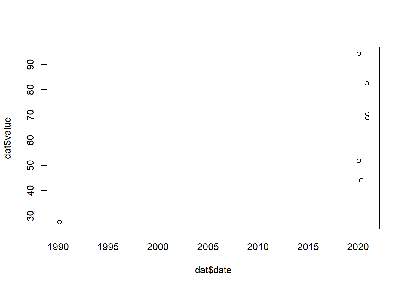
What about date2, which is the same information just organized differently?
dat$date2
#> [1] "2.2020.05"  "3.2020.12"  "29.2020.01" "11.2020.11"
#> [5] "01-1990-03" "03.2020.12" "29.2020.01"
The command is just whatever order the things are in:
dym(dat$date2)
#> [1] "2020-05-02" "2020-12-03" "2020-01-29" "2020-11-11"
#> [5] "1990-03-01" "2020-12-03" "2020-01-29"
Another way we could make use of this date infomration is to have a day, year, and month column.
Let’s first use gsub to change the dashes to periods in the one weird one. For some reason we don’t have to use square brackets around a period when it’s what we are replacing with. I KNOW. I’M MAD TOO.
dat$date3 <- gsub("-",".", dat$date1)
dat$date3
#> [1] "2020.05.2"  "2020.12.03" "2020.01.29" "2020.11.11"
#> [5] "1990.03.01" "2020.12.03" "2020.01.29"
Then we can make use of the separate function from the tidyr package.
We will first have to install that package:
#install.packages("tidyr")For the seperate command we give it the full dataset, the column we want to separate, what we want to name the new columns that are generated, and what the “seperator” in the column is.
I’m going to give you a shortcut/alternative to loading a package if you are only using one command. If we want to use one command from a package without loading the whole thing, we can tell it the package name and put two colons, and then it will allow us to use that function:
tidyr::separate(dat,
                col="date3",
                into=c("year","month","day"),
                sep="[.]")
#>   state      date1      date2       date    value year
#> 1    AL  2020.05.2  2.2020.05 2020-05-02 44.16195 2020
#> 2    AZ 2020.12.03  3.2020.12 2020-12-03 68.79357 2020
#> 3    CA 2020.01.29 29.2020.01 2020-01-29 94.25560 2020
#> 4    FL 2020.11.11 11.2020.11 2020-11-11 82.50894 2020
#> 5    GA 1990-03-01 01-1990-03 1990-03-01 27.42534 1990
#> 6    KY 2020.12.03 03.2020.12 2020-12-03 70.49424 2020
#> 7    MN 2020.01.29 29.2020.01 2020-01-29 51.82528 2020
#>   month day
#> 1    05   2
#> 2    12  03
#> 3    01  29
#> 4    11  11
#> 5    03  01
#> 6    12  03
#> 7    01  29
First: how did I know to use the square brackets around the period this time? Because I tried to do it without and it didn’t work! Notice also that this function returns our whole dataset with the new columns appended on. As such, to save this we have to overwrite the dataframe:
Notive also that this time I just fully omitted the sep argument. The separate function will take a guess at what the seperator of the information is, and here it correctly sees that is the period. I don’t rely on this, but it’s a good shortcut!
OK great, what is the average of the day column?
#Uncomment this
mean(dat.new$day)
#> Warning in mean.default(dat.new$day): argument is not
#> numeric or logical: returning NA
#> [1] NA
What’s happening here? Well if we look:
class(dat.new$day)
#> [1] "character"
This is still being treated as text! We can easily convert these to numeric:
dat.new$year <- as.numeric(dat.new$year)
dat.new$month <- as.numeric(dat.new$month)
dat.new$day <- as.numeric(dat.new$day)

mean(dat.new$day)
#> [1] 11.14286