30 CIs and tests: comparing two means

You have learnt to ask a RQ, design a study, classify and summarise the data, construct confidence intervals, and conduct hypothesis tests. In this chapter, you will learn to:

• identify situations where comparing two means is appropriate.
• construct confidence intervals for the difference between two independent means.
• conduct hypothesis tests for comparing two means.
• determine whether the conditions for using these methods apply in a given situation.

30.1 Introduction: garter snakes

Some Mexican garter snakes (Thamnophis melanogaster) live in habitats with no crayfish, while some live in habitats with crayfish and hence use crayfish as a food source. Manjarrez, Macias Garcia, and Drummond (2017) were interested in whether the snakes in these two regions were different:

For female Mexican garter snakes, is the mean snout--vent length (SVL) different for those in regions with crayfish and without crayfish?

Two different groups of snakes are studied, so this is a relational RQ with no intervention (the study uses a between-individuals comparison), and the data are shown below.

30.2 Summarising the data and error bar charts

A numerical summary must summarise the difference between the means, because the RQ is about this difference. Both groups should be summarised too. The information can be found using software (Fig. 30.1), and compiled into a table (Table 30.1). The appropriate summary for graphically summarising the data is (for example) a boxplot (Fig. 30.2, left panel).

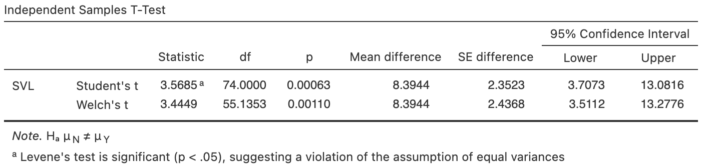
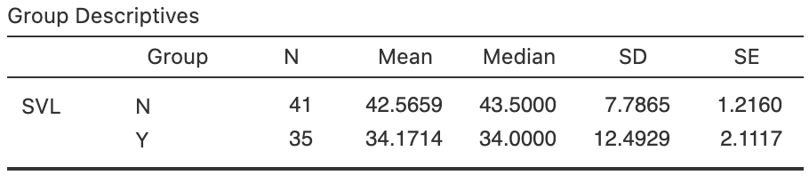
FIGURE 30.1: Software output for the garter-snakes data.

TABLE 30.1: Numerical summaries of SVL (in cm) for female snakes in two regions.

	Mean	Standard deviation	Sample size	Standard error
Non-crayfish region	\(42.57\)	\(\phantom{0}7.79\)	\(41\)	\(1.216\)
Crayfish region	\(34.17\)	\(12.49\)	\(35\)	\(2.112\)
Difference	\(\phantom{0}8.39\)			\(2.437\)

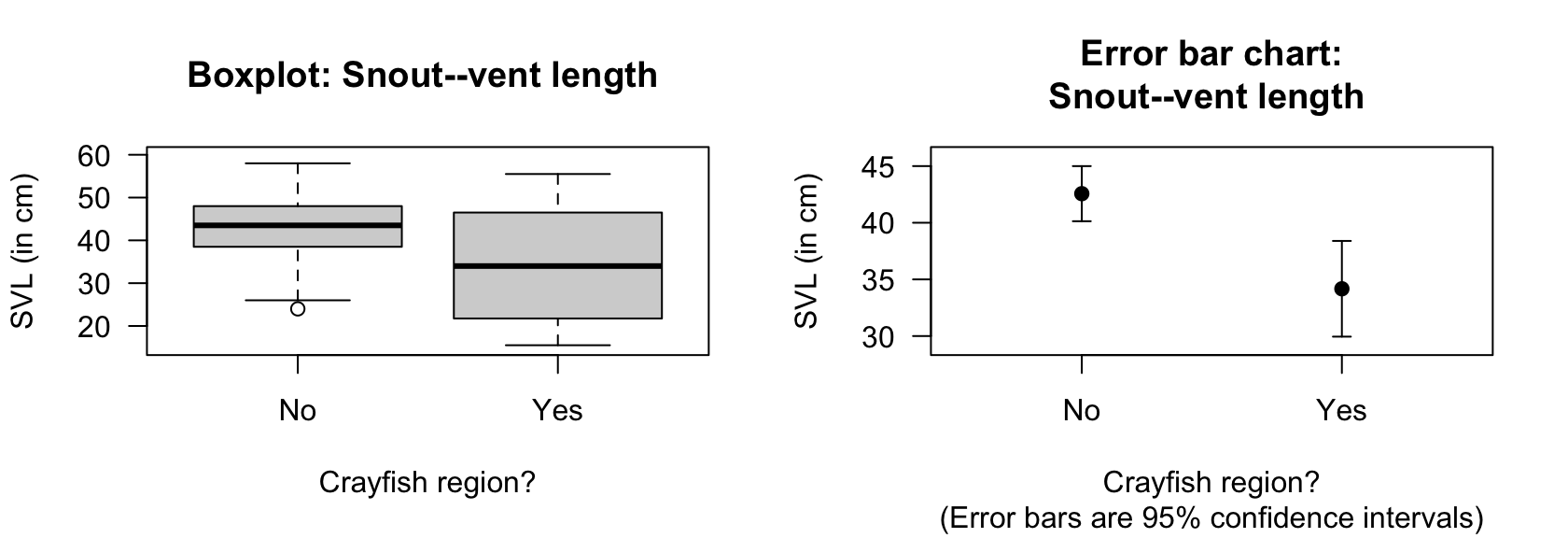
FIGURE 30.2: Boxplot (left) and error bar chart (right) of SVL for female snakes in two regions.

Since two groups are being compared, subscripts are used to distinguish between the statistics for the two groups; say, Groups \(1\) and \(2\) in general (Table 30.2). Using this notation, the parameter in the RQ is the difference between population means: \(\mu_1 - \mu_2\). As usual, the population values are unknown, so this is estimated using the statistic \(\bar{x}_1 - \bar{x}_2\).

TABLE 30.2: Notation used to distinguish between the two independent groups.

	Group 1	Group 2	Comparing groups
Sample sizes:	\(n_1\)	\(n_2\)
Population means:	\(\mu_1\)	\(\mu_2\)	\(\mu_1 - \mu_2\)
Sample means:	\(\bar{x}_1\)	\(\bar{x}_2\)	\(\bar{x}_1 - \bar{x}_2\)
Standard deviations:	\(s_1\)	\(s_2\)
Standard errors:	\(\displaystyle\text{s.e.}(\bar{x}_1) = \frac{s_1}{\sqrt{n_1}}\)	\(\displaystyle\text{s.e.}(\bar{x}_2) = \frac{s_2}{\sqrt{n_2}}\)	\(\displaystyle\text{s.e.}(\bar{x}_1 - \bar{x}_2)\)

For the garter-snakes data, define the differences as the mean for females snakes living in non-crayfish regions (\(N\)), minus the mean for female snakes in crayfish regions (\(C\)): \(\mu_N - \mu_C\). This is the parameter. By this definition, the differences refer to how much larger (on average) the SVL is for snakes living in non-crayfish regions.

Here the difference is computed as the mean SVL for snakes living in non-crayfish regions, minus the mean SVL for snakes living in crayfish regions. Computing the difference as the mean SVL for snakes in crayfish regions, minus non-crayfish regions is also correct.

You need to be clear about how the difference is computed, and be consistent throughout. The meaning of the conclusions will be the same whichever direction is used.

A useful way to compare the means of two (or more) groups is to display the CIs for the means of the groups being compared in an error bar chart. Error bars charts display the expected variation in the sample means from sample to sample, while boxplots display the variation in the individual observations. For the garter-snakes data, the error bar chart (Fig. 30.2, right panel) shows the \(95\)% CI for each group; the mean has been added as a dot.

The two CIs for the SVL are (using information from the bottom table in Fig. 30.1):

• \(34.171 \pm (2 \times 2.112)\), or from \(29.94\) to \(38.40\,\text{cm}\).
• \(42.566 \pm (2\times 1.216)\), or from \(40.13\) to \(45.00\,\text{cm}\).

However, the error bar chart, and these CIs, do not give a CI for the difference between the two means, as relevant to the RQ.

Example 30.1 (Error bar charts) Schepaschenko et al. (2017a) studied the foliage biomass of small-leaved lime trees from three sources: coppices; natural; planted. Three graphical summaries are shown in Fig. 30.3: a boxplot (showing the variation in individual trees; left), an error bar chart (showing the variation in the sample means; centre) on the same vertical scale as the boxplot, and the same error bar chart using a more appropriate scale for the error bar plot (right).

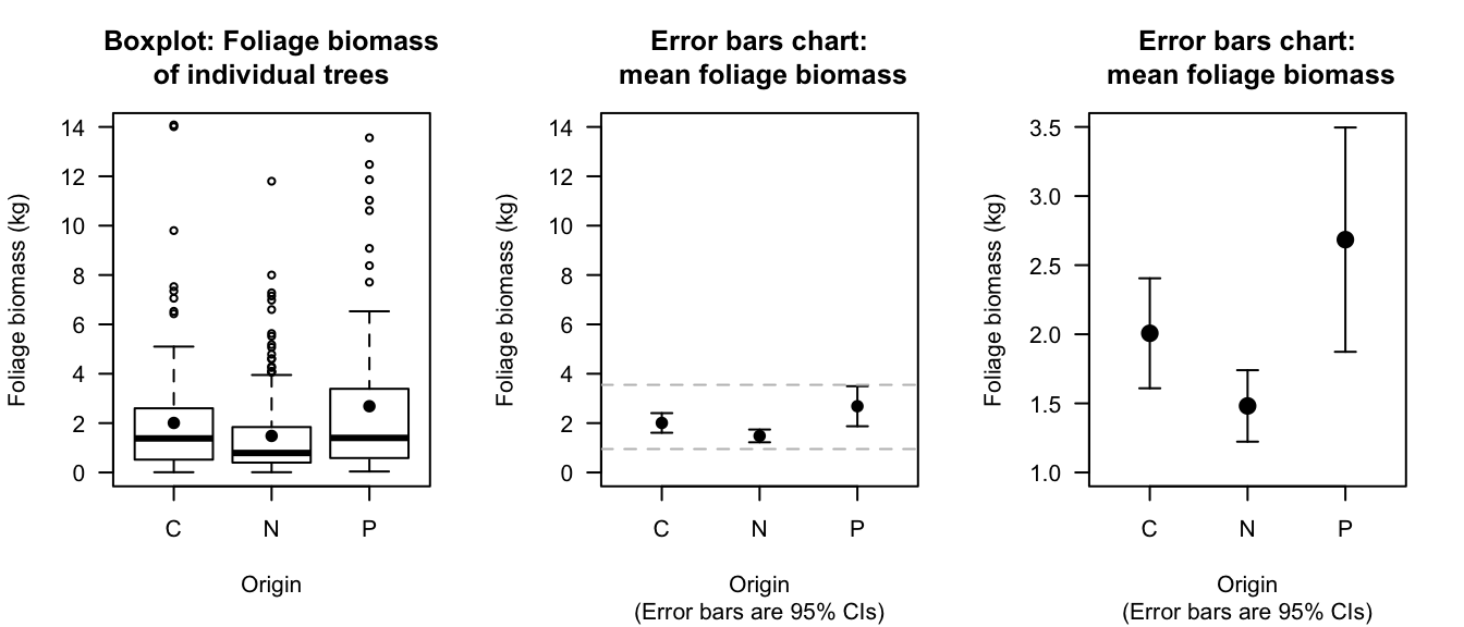
FIGURE 30.3: Boxplot (left) and error bar charts (centre; right) comparing the mean foliage biomass for small-leaved lime trees from three sources (C: Coppice; N: Natural; P: Planted). The centre panel shows an error bar chart using the same vertical scale as the boxplot; the dashed horizontal lines are the limits of the error bar chart on the right. The right error bar chart uses a more appropriate scale on the vertical axis. The solid dots show the mean of the distributions.

30.3 Confidence intervals for \(\mu_1 - \mu_2\)

Each sample will comprise different snakes, and give different SVLs. The sample means for each group will differ from sample to sample, and the difference between the sample means will be different for each sample. The difference between the sample means varies from sample to sample, and so has a sampling distribution and a standard error.

Definition 30.1 (Sampling distribution for the difference between two sample means) The sampling distribution of the difference between two sample means \(\bar{x}_1\) and \(\bar{x}_2\) is (when the appropriate conditions are met; Sect. 30.5) described by:

• an approximate normal distribution,
• centred around a sampling mean whose value is \({\mu_1} - {\mu_2}\), the difference between the population means,
• with a standard deviation, called the standard error of the difference between the means, of \(\displaystyle\text{s.e.}(\bar{x}_1 - \bar{x}_2)\).

The standard error for the difference between the means is found using \[ \text{s.e.}(\bar{x}_1 - \bar{x}_2) = \sqrt{ \text{s.e.}(\bar{x}_1)^2 + \text{s.e.}(\bar{x}_2)^2}, \] though this value will often be given (e.g., on computer output) rather than needing to be computed.

For the garter-snakes data, the differences between the sample means will have:

• an approximate normal distribution,
• centred around the sampling mean whose value is \(\mu_N - \mu_C\),
• with a standard deviation, called the standard error of the difference, of \(\text{s.e.}(\bar{x}_P - \bar{x}_C) = 2.437\).

The standard error of the difference between the means was computed using \[ \text{s.e.}(\bar{x}_N - \bar{x}_C) = \sqrt{ \text{s.e.}(\bar{x}_N)^2 + \text{s.e.}(\bar{x}_C)^2} = \sqrt{ 1.216^2 + 2.1112^2 } = 2.437, \] the same value shown in the second row of the software output (Fig. 30.1).

The sampling distribution describes how the values of \(\bar{x}_N - \bar{x}_C\) vary from sample to sample. Then, finding a \(95\)% CI for the difference between the mean SVLs is similar to the process used in Chap. 23, since the sampling distribution has an approximate normal distribution: \[ \text{statistic} \pm \big(\text{multiplier} \times\text{s.e.}(\text{statistic})\big). \] When the statistic is \(\bar{x}_P - \bar{x}_C\), the approximate \(95\)% CI is \[ (\bar{x}_N - \bar{x}_C) \pm \big(2 \times \text{s.e.}(\bar{x}_N - \bar{x}_C)\big). \] So, in this case, the approximate \(95\)% CI is \[ 8.394 \pm (2 \times 2.437) \] or \(8.394\pm 4.874\), after rounding appropriately. We write:

The difference between mean SVLs is \(8.39\,\text{cm}\), shorter for those living in a crayfish region (mean: \(34.17\,\text{cm}\); s.e.: \(2.112\); \(n = 35\)) compared to those not living in a crayfish region (mean: \(42.57\,\text{cm}\); s.e.: \(1.216\); \(n = 41\)), with an approximate \(95\)% CI for the difference between mean SVLs from \(3.52\) to \(13.27\,\text{cm}\).

The plausible values for the difference between the two population means SVLs are between \(3.52\) to \(13.27\,\text{cm}\) (shorter for those living in crayfish regions).

Giving the CI alone is insufficient; the direction in which the differences were calculated must be given, so readers know which group had the higher mean.

Output from software often shows two CIs for the difference between the two means (Fig. 30.1). We will use the results from Welch's test (the second row), as this row of output is more general, and makes fewer assumptions. The information in the second row makes fewer assumptions, and is more widely applicable.

Most software gives two confidence intervals: one assuming the standard deviations in the two groups are the same (Student's), and another not assuming the standard deviations in the two groups are the same (Welch's).

We will use the information that does not assume the standard deviations in the two groups are the same. In the software output in Fig. 30.1, this is the second row of the top table (labelled 'Welch's \(t\)'). (The information in both rows are often similar anyway.)

From the output, the \(95\)% CI for the difference is from \(3.51\) to \(13.28\,\text{cm}\). The approximate CI and the exact (from software) CIs are only slightly different, as the samples sizes are not too small. (Recall: the \(t\)-multiplier of \(2\) is an approximation, based on the \(68\)--\(95\)--\(99.7\) rule.)

30.4 Hypothesis tests for \(\mu_1 - \mu_2\): \(t\)-test

As always, the null hypothesis is the default 'no difference, no change, no relationship' position; any difference between the parameter and statistic is due to sampling variation (Sect. 28.2). Hence, the null hypothesis is 'no difference' between the population mean SVL of the two groups:

• \(H_0\): \(\mu_N - \mu_C = 0\) (equivalent to \(\mu_N = \mu_C\)).

From the RQ, the alternative hypothesis is two-tailed:

• \(H_1\): \(\mu_N - \mu_C\ne 0\) (equivalent to \(\mu_N \ne \mu_C\)).

The alternative hypothesis proposes that any difference between the sample means is because a difference really exists between the population means. The alternative hypothesis is two-tailed, based on the RQ.

The difference between the sample mean SVLs in the two groups depends on which one of the many possible samples is randomly obtained, even if the difference between the means in the population is zero. The difference between the sample means is \(8.394\,\text{cm}\), but this difference will vary from sample to sample; that is, sampling variation exists.

For the SVL data, the sampling distribution of \(\bar{x}_N - \bar{x}_C\) can be described as (see Def. 30.1):

• an approximate normal distribution,
• centred around the sampling mean whose value is \({\mu_{N}} - {\mu_{C}} = 0\), the difference between the population means (from \(H_0\)),
• with a standard deviation of \(\text{s.e.}(\bar{x}_N - \bar{x}_C) = 2.4368\).

Most software gives two hypothesis test results: one assuming the standard deviations in the two groups are the same, and another not assuming the standard deviations in the two groups are the same.

We will use the information that does not assume the standard deviations in the two groups are the same. In the software output in Fig. 30.1, this is the second row of the bottom table (labelled 'Welch's \(t\)'). (The information in both rows are often similar anyway.)

The observed difference between sample means, relative to what was expected, is found by computing the test statistic; in this case, a \(t\)-score. The software output (Fig. 30.1) gives the \(t\)-score, but the \(t\)-score can also be computed using the information in Table 30.1: \[\begin{align*} t &= \frac{\text{sample statistic} - \text{mean of sampling distribution (from $H_0$)}} {\text{standard deviation of sampling distribution}}\\[6pt] &= \frac{ (\bar{x}_P - \bar{x}_C) - (\mu_P - \mu_C)} {\text{s.e.}(\bar{x}_P - \bar{x}_C)} = \frac{8.39 - 0}{2.4368} = 3.44, \end{align*}\] as in the software output.

A \(P\)-value determines if the sample statistic is consistent with the assumption (i.e., \(H_0\)). Since the \(t\)-score is large, the \(P\)-value will be small using the \(68\)--\(95\)--\(99.7\) rule (and less than \(0.003\)). This is confirmed by the software (Fig. 30.1): the two-tailed \(P\)-value is \(0.0011\).

A small \(P\)-value suggests the observations are inconsistent with the assumption of no difference (Table 28.1), and the difference between the sample means could not be reasonably explained by sampling variation, if \(\mu_N - \mu_C = 0\).

Click on the pins in the following image, and describe what the software output tells us.

In conclusion, write:

Strong evidence exists in the sample (two independent samples \(t = 3.445\); two-tailed \(P = 0.0011\)) that the population mean SVL is different for female snakes living in crayfish regions (mean: \(34.17\cm\); \(n = 35\)) and non-crayfish regions (mean: \(42.57\,\text{cm}\); \(n = 41\); \(95\)% CI for the difference: \(3.51\) to \(13.28\,\text{cm}\) longer for those in non-crayfish regions).

The conclusion contains an answer to the RQ, the evidence leading to this conclusion (\(t = 3.44\); two-tailed \(P = 0.0011\)), and sample summary statistics, including a CI.

30.5 Statistical validity conditions

As usual, these results apply under certain conditions. Statistical validity can be assessed using these criteria:

• When both samples have \(n \ge 25\), the test is statistically valid. (If the distribution of a sample is highly skewed, the sample size for that sample may need to be larger.)
• When one or both groups have \(25\) or fewer observations, the test is statistically valid only if the populations corresponding to both comparison groups have an approximate normal distribution.

The sample size of \(25\) is a rough figure; some books give other values (such as \(30\)).

This condition ensures that the distribution of the difference between sample means has an approximate normal distribution (so that, for example, the \(68\)--\(95\)--\(99.7\) rule can be used). The histograms of the sample data can be used to determine if normality of the populations seems reasonable. The units of analysis are also assumed to be independent (e.g., from a simple random sample).

If the statistical validity conditions are not met, other similar options include using a Mann-Whitney test (Conover 2003) or using resampling methods (Efron and Hastie 2021).

Example 30.2 (Statistical validity) For the garter-snakes data, both samples sizes exceed \(25\) (\(41\) and \(35\)), so the test is statistically valid. The data in each group do not need to be normally distributed, since both sample sizes are larger than \(25\), and the data are not severely skewed (Fig. 30.2, left panel).

30.6 Tests for comparing more than two means: ANOVA

Often, more than two means need to be compared. This requires a different method, called analysis of variance (or anova). The details are beyond the scope of this book. In this section, a very brief overview of using a one-way anova is given, using an example. Importantly, this example shows that the basic principles of hypothesis testing from Chap. 28 still apply.

Example 30.3 (ANOVA) [Dataset: BMI] E. Johnson, Millar, and Shiely (2021) collected data from hospital outpatients at an Irish hospital (Table 30.3). One research question involves comparing the mean number of days per week that patients exercise for more than \(30\,\text{mins}\) (say, \(\mu\)) according to their smoking status: daily (\(D\)), occasionally (\(O\)) or not at all (\(N\)). An error bar chart can be used to display the three groups (Fig. 30.4).

As per Sect. 28.2, the null hypothesis is 'no difference' between the population means: \[ \text{$H_0$:}\ \mu_D = \mu_O = \mu_N. \] The alternative hypothesis is that the three means are not all equal. This hypothesis encompasses many possibilities: for example, that the three means are all different from each other, or that the first is different from the other two (which are the same). Because the alternative hypothesis encompasses many possibilities, it is difficult to write using symbols, so we write: \[ \text{$H_1$:}\ \text{Not all means are equal.} \]

For comparing more than two mean, the alternative hypothesis is always two-tailed.

Performing an anova using software (Fig. 30.5) gives \(P = 0.00007\). (The test statistic here is an \(F\)-score; we don't discuss these further.) The \(P\)-value in this context means the same as usual (Sect. 28.6): there is very strong evidence to support the alternative hypothesis (that the three means are not all equal).

While we know the means are not all the same, we do not know which group means are different from which other group means. One option might be to compare all possible combinations of two groups (i.e., the means of groups \(D\) and \(O\); the means of groups \(D\) and \(N\); the means of groups \(O\) and \(N\)) using three separate two-sample \(t\)-tests. However, this approach increases the probability of declaring a false positive (i.e., of making a Type I error; Sect. 28.7): incorrectly declaring a difference between two sets of means. The correct approach requires methods beyond this book.

TABLE 30.3: Number of days per week where patients do more than \(30\) mins of exercise.

Smokes daily	\(1.27\)	\(0.79\)	\(0.237\)	\(11\)
Smokes occasionally	\(2.77\)	\(1.64\)	\(0.455\)	\(13\)
Does not smoke	\(3.15\)	\(1.93\)	\(0.285\)	\(46\)

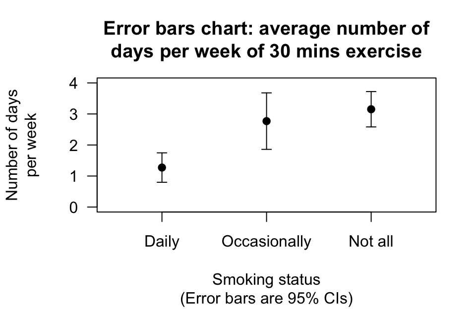
FIGURE 30.4: The error bar chart for comparing the number of days per week on which people do more than \(30\,\text{mins}\) of exercise, for different smoking groups.

Anova is a general tool that can be extended beyond just comparing more than two means, and used in many and varied context for the analysis of data.

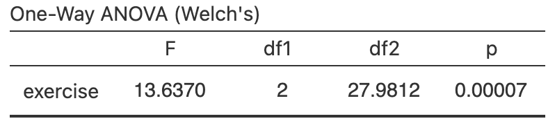
FIGURE 30.5: Software output for testing hypotheses for the BMI data.

30.7 Example: speed signage

To reduce vehicle speeds on freeway exit ramps, Ma et al. (2019) studied adding additional signage. At one site (Ningxuan Freeway), speeds were recorded for \(38\) vehicles before the extra signage was added, and then for \(41\) different vehicles after the extra signage was added.

The researchers are hoping that the addition of extra signage will reduce the mean speed of the vehicles. The RQ is:

At this freeway exit, does the mean vehicle speed reduce after extra signage is added?

The data are not paired: different vehicles are measured before (\(B\)) and after (\(A\)) the extra signage is added. Define \(\mu\) as the mean speed (in km.h^\(-1\)) on the exit ramp, and the parameter as \(\mu_B - \mu_A\), the reduction in the mean speed.

The data can be summarised (Table 30.4) using the software output (Fig. 30.6), where \[ \text{s.e.}(\bar{x}_B - \bar{x}_A) = \sqrt{ \text{s.e.}(\bar{x}_B)^2 + \text{s.e.}(\bar{x}_A)^2} = \sqrt{ 2.140^2 + 2.051^2} = 2.965, \] as in the output table (Row 2). A boxplot of the data is shown in Fig. 30.7 (left panel), and an error bar chart in Fig. 30.7 (right panel).

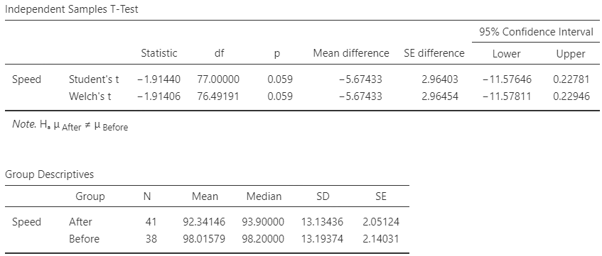
FIGURE 30.6: Software output for the speed data.

TABLE 30.4: The signage data summary (in km.h\(^{-1}\)).

	Mean	Median	Standard deviation	Standard error	Sample size
Before	\(98.02\)	\(98.2\)	\(13.194\)	\(\phantom{0}2.1\)	\(38\)
After	\(92.34\)	\(93.9\)	\(13.134\)	\(\phantom{0}2.1\)	\(41\)
Speed reduction	\(\phantom{0}5.68\)			\(\phantom{0}3.0\)

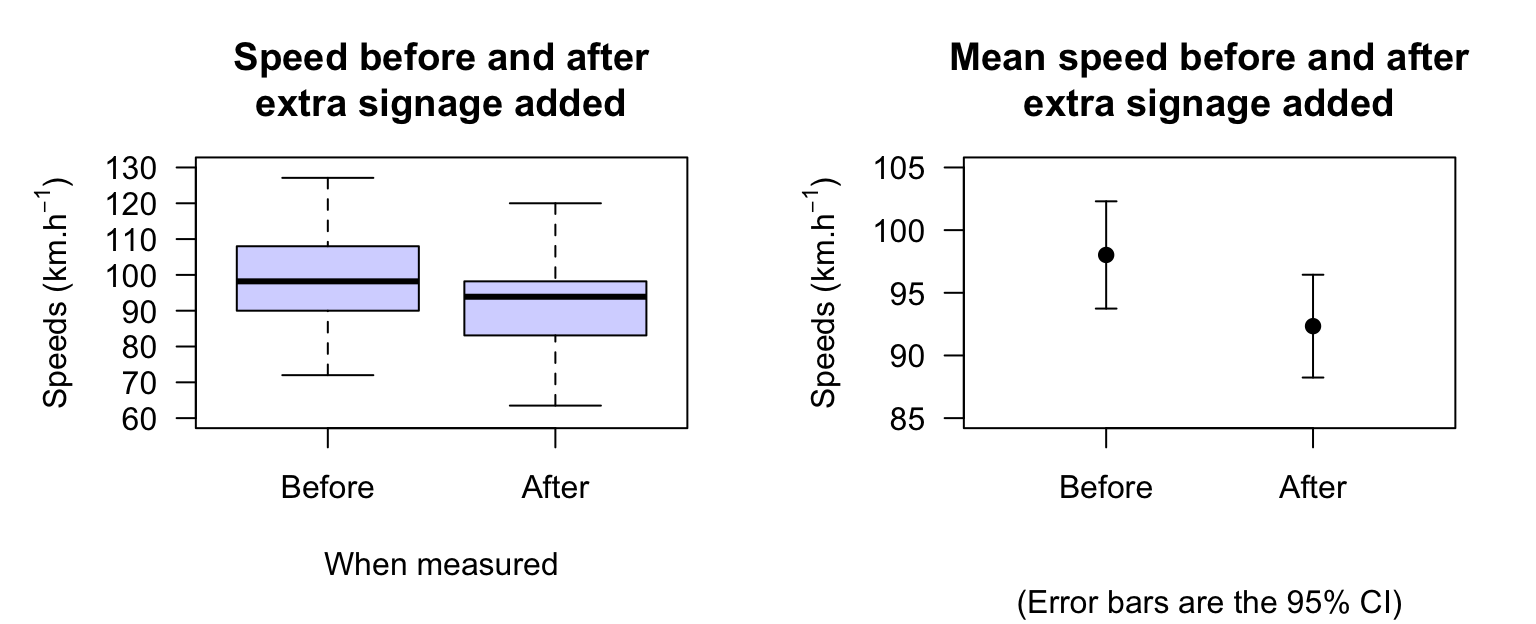
FIGURE 30.7: Boxplot (left) and error bar chart (right) showing the mean speed before and after the addition of extra signage, and the \(95\)% CIs. The vertical scales on the two graphs are different.

Define \(\mu\) as the mean speed (in km.h^\(-1\)) on the exit ramp. Then, the parameter is \(\mu_B - \mu_A\), the reduction in the population mean speed after signage is added. An approximate \(95\)% CI for the difference between the mean speeds is \[ 5.674 \pm (2 \times 2.9642), \] or from \(-0.25\) to \(11.60\,\text{km}\).h^\(-1\). (This is very similar to the \(95\)% CI shown in Fig. 30.6.) The negative value is not a negative speed. Since the difference between the means is defined as a reduction, this CI means that the reduction in the populations mean speed is likely between \(-0.25\) to \(11.64\,\text{km}\).h^\(-1\). Since a negative reduction is an increase, this is more easily understood as the difference being located between a \(0.25\,\text{km}\).h^\(-1\)increase before the signage was added to an \(11.64\,\text{km}\).h^\(-1\)reduction after the signage was added.

The hypotheses are:

• \(H_0\): \(\mu_B - \mu_A = 0\): there is no difference in the population mean speeds.
• \(H_1\): \(\mu_B - \mu_A > 0\): the population mean speed has reduced after the addition of signage.

The best estimate of the difference in population means is the difference between the sample means: \((\bar{x}_B - \bar{x}_A) = 5.68\). Since \(\text{s.e.}(\bar{x}_B - \bar{x}_A) = 2.965\), the \(t\)-score is \[ t = \frac{(\bar{x}_B - \bar{x}_A) - (\mu_B - \mu_A)}{\text{s.e.}(\bar{x}_B - \bar{x}_{A})} = \frac{5.674 - 0}{2.9642} = 1.91. \] using Eq. (27.1). (Recall that \(\mu_B - \mu_A = 0\) is initially assumed, from the null hypothesis.)

Remembering that the alternative hypothesis is one-tailed, the \(P\)-value (using the \(68\)--\(95\)--\(99.7\) rule) is larger than \(0.025\), but smaller than \(0.32\), so making a clear decision is difficult without using software. However, since the \(t\)-score is just less than 2, we suspect that the \(P\)-value is likely to be closer to \(0.025\) than to \(0.32\).

From software, \(P = 0.0297\) (you cannot be this precise just using the \(68\)--\(95\)--\(99.7\) rule). Using Table 28.1, this \(P\)-value provides moderate evidence of a reduction in mean speeds. We conclude:

Moderate evidence exists in the sample (\(t = 1.91\); one-tailed \(P = 0.030\)) that mean speeds have reduced after the addition of extra signage (mean reduction: \(5.67\,\text{km}\).h^\(-1\); \(95\)% CI for the difference: \(-0.23\) to \(11.6\,\text{km}\).h^\(-1\); s.e.: \(2.96\,\text{km}\).h^\(-1\)). The before mean speed was \(98.02\,\text{km}\).h^\(-1\) (\(n = 38\); standard deviation: \(13.19\,\text{km}\).h^\(-1\)); the after mean speed was \(92.34\,\text{km}\).h^\(-1\) (\(n = 41\); standard deviation: \(13.13\,\text{km}\).h^\(-1\)).

Whether the mean speed reduction of \(5.67\,\text{km}\).h^\(-1\) has practical importance is a separate issue. Using the validity conditions, the CI and the test are statistically valid.

Remember: the conclusion must make clear which mean is larger!

30.8 Example: chamomile tea

(This study was seen in Sect. 29.8.) Rafraf, Zemestani, and Asghari-Jafarabadi (2015) studied patients with Type 2 diabetes mellitus (T2DM). They randomly allocated \(32\) patients into a control group (who drank hot water), and \(32\) to receive chamomile tea (Rafraf, Zemestani, and Asghari-Jafarabadi (2015)).

The total glucose (TG) was measured for each individual in both groups, both before the intervention and after eight weeks on the intervention. Summary data are given in Table 29.4. Evidence suggests that the chamomile tea group shows a mean reduction in TG (Sect. 29.8), while the hot-water group shows no evidence of a reduction. That is, there appears to be a difference between the two groups regarding the change in TG. However, the differences between the chamomile-tea and the hot-water groups may be due to the samples selected (i.e., sampling variation), so comparing the changes between the two groups is helpful.

The following relational RQ can be asked:

For patients with T2DM, is the mean reduction in TG greater for the chamomile tea group compared to the hot water group?

Notice the RQ is one-tailed; the aim of the study is to determine if the chamomile-tea drinking group performs better (i.e., reduces the mean TG) than the control group.

This RQ is comparing two separate groups; specifically, comparing the differences between the two groups. This study contains both within-individuals comparisons (see Sect. 29.8) and a between-individuals comparison (this section); see Fig. 30.8. This is equivalent to treating the differences for both groups as the two separate sets of data in the two-sample analysis.

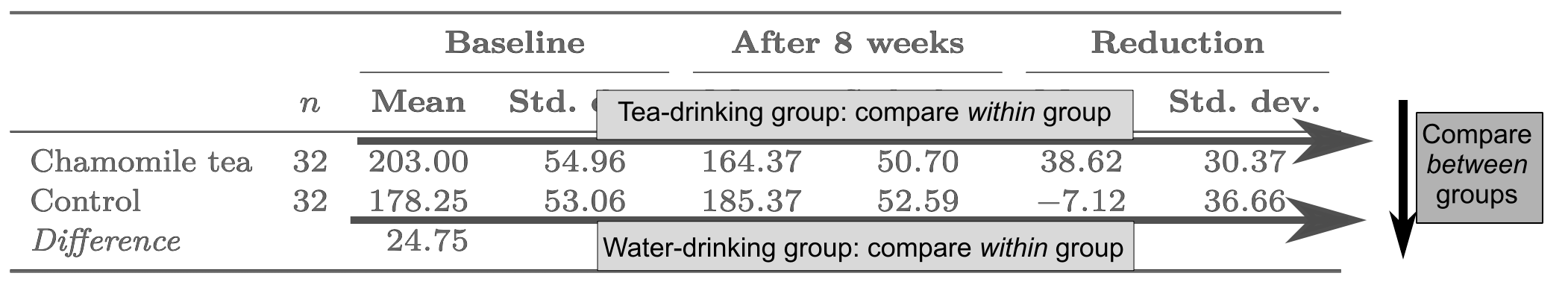
FIGURE 30.8: The chamomile-tea study has two within-individuals comparisons, and a between-individuals comparison.

The corresponding hypotheses are:

\[ \text{$H_0$: $\mu_T - \mu_W = 0$ and $H_1$: $\mu_T - \mu_W > 0$} \]

where \(\mu\) refers to the mean reduction in TG, \(T\) refers to the tea-drinking group, and \(W\) to the hot-water drinking group.

The parameter \(\mu_T - \mu_W\) is estimated by the statistic \(\bar{x}_T - \bar{x}_W = 45.74\,\text{mg}\).dl^\(-1\). The standard error for the statistic was found as \(\text{s.e.}(\bar{x}_T - \bar{x}_W) = 8.42\) (using the information in Table 29.4). Hence, the test statistic is: \[ t = \frac{(\mu_T - \mu_W) - (\bar{x}_T - \bar{x}_W)}{\text{s.e.}(\bar{x}_T - \bar{x}_W)} = \frac{45.75 - 0}{8.42} = 5.43, \] which is very large, so the \(P\) value will be very small (using the \(68\)--\(95\)--\(99.7\) rule), and certainly smaller than \(0.001\).

We write:

There is very strong evidence (\(t = 5.43\); one-tailed \(P < 0.001\)) that the mean reduction in TG for the chamomile-tea drinking group (mean reduction: \(36.62\,\text{mg}\).dl^\(-1\)) is greater than the mean reduction in TG for the hot-water drinking group (mean reduction: \(-7.12\,\text{mg}\).dl^\(-1\); difference between means: \(45.74\,\text{mg}\).dl^\(-1\); approx. \(95\)% CI: \(28.64\) to \(62.84\,\text{mg}\).dl^\(-1\)).

Again, the sample sizes are larger than \(25\), so the results are statistically valid.

30.9 Chapter summary

To compute a confidence interval (CI) for the difference between two means, compute the difference between the two sample mean, \(\bar{x}_1 - \bar{x}_2\), and identify the sample sizes \(n_1\) and \(n_2\). Then compute the standard error, which quantifies how much the value of \(\bar{x}_1 - \bar{x}_2\) varies across all possible samples: \[ \text{s.e.}(\bar{x}_1 - \bar{x}_2) = \sqrt{ \text{s.e}(\bar{x}_1) + \text{s.e.}(\bar{x}_2)}, \] where \(\text{s.e.}(\bar{x}_1)\) and \(\text{s.e.}(\bar{x}_2)\) are the standard errors of Groups \(1\) and \(2\). The margin of error is (multiplier\({}\times{}\)standard error), where the multiplier is \(2\) for an approximate \(95\)% CI (using the \(68\)--\(95\)--\(99.7\) rule). Then the CI is: \[ (\bar{x}_1 - \bar{x}_2) \pm \left( \text{multiplier}\times\text{standard error} \right). \] The statistical validity conditions should also be checked.

To test a hypothesis about a difference between two population means \(\mu_1 - \mu_2\):

• Write the null hypothesis (\(H_0\)) and the alternative hypothesis (\(H_1\)).
• Initially assume the value of \((\mu_1 - \mu_2)\) in the null hypothesis to be true.
• Then, describe the sampling distribution, which describes what to expect from the difference between the sample means based on this assumption: under certain statistical validity conditions, the difference between the sample means vary with:
• an approximate normal distribution,
• with sampling mean whose value is the value of \((\mu_1 - \mu_2)\) (from \(H_0\)), and
• having a standard deviation of \(\displaystyle \text{s.e.}(\bar{x}_1 - \bar{x}_2)\).
• Compute the value of the test statistic: \[ t = \frac{ (\bar{x}_1 - \bar{x}_2) - (\mu_1 - \mu_2)}{\text{s.e.}(\bar{x}_1 - \bar{x}_2)}, \] where \(\mu_1 - \mu_2\) is the hypothesised difference given in the null hypothesis.
• The \(t\)-value is like a \(z\)-score, and so an approximate \(P\)-value can be estimated using the \(68\)--\(95\)--\(99.7\) rule, or found using software.
• Make a decision, and write a conclusion.
• Check the statistical validity conditions.

Anova is used to compare means for more than two groups.

The following short video may help explain some of these concepts:

30.10 Quick review questions

Y.-M. Lee et al. (2016) studied iron levels in Koreans with Type II diabetes, comparing people on a vegan (\(n = 46\)) and a conventional (\(n = 47\)) diet for \(12\) weeks. A summary of the data for iron levels are shown in Table 30.5.

Are the following statements true or false?

1. An appropriate graph for displaying the data is a boxplot. TRUE FALSE
2. The difference between the means in the population is denoted \(\mu_V - \mu_C\), where \(V\) represent the vegan diet, and \(C\) represents the conventional diet.
   TRUE FALSE
3. The standard error of the difference between the sample means is denoted \(\text{s.e.}(\bar{x}_V) - \text{s.e.}(\bar{x}_C)\).
   TRUE FALSE
4. An error bar chart displays the variation in the data.
   TRUE FALSE
5. The sample size is missing from the Difference row, but the value is \(47 - 46 = 1\). TRUE FALSE
6. The standard deviation is missing from the Difference row, but the value is \(0.4\). TRUE FALSE
7. The standard error is missing from the Difference row, but there is not enough information to compute its value. TRUE FALSE
8. The two-tailed \(P\)-value for the comparison is given as \(P = 0.046\). This means that no evidence that the population means are different TRUE FALSE

TABLE 30.5: Comparing the iron levels (mg) for subjects using a vegan or conventional diet for \(12\) weeks.

	Mean	Standard deviation	\(n\)
Vegan diet	\(13.9\)	\(2.3\)	\(46\)
Conventional diet	\(15.0\)	\(2.7\)	\(47\)
Difference	\(\phantom{0}1.1\)

30.11 Exercises

Answers to odd-numbered exercises are given at the end of the book.

Exercise 30.1 Suppose researchers are comparing the cell diameter of lymphocytes (a type of white blood cell) and tumour cells. Define the mean diameter of lymphocytes as \(\mu_L\), and the mean diameter of tumour cells as \(\mu_T\).

If the difference between the means were defined as \(\mu_L - \mu_T\), what does this mean?

Exercise 30.2 Suppose researchers are comparing the braking distance of cars using two different types of brake pads (Type A and Type B). Define the mean breaking distance for cars with Type A brake pads as \(\mu_A\), and mean breaking distance for cars with Type B brake pads as \(\mu_B\).

If the difference between the means were defined as \(\mu_B - \mu_A\), what does this mean?

Exercise 30.3 Sketch the sampling distribution for the difference between the mean speeds before and after adding extra signage (Sect. 30.7).

Exercise 30.4 Sketch the sampling distribution for the difference between reduction in mean TG for the tea-drinking and the hot-water drinking group (Sect. 30.8).

Exercise 30.5 Agbayani, Fortune, and Trites (2020) measured (among other things) the length of gray whales (Eschrichtius robustus) at birth. Are female gray whales longer than males, on average, in the population at birth? Summary information is shown in Table 30.6.

TABLE 30.6: Numerical summary of length of whales at birth (in m).

	Mean	Standard deviation	Sample size
Female	\(4.66\)	\(0.38\)	\(26\)
Male	\(4.60\)	\(0.30\)	\(30\)

1. Define the parameter, and write down its estimate. Carefully describe what it means.
2. Sketch an error bar chart.
3. Compute the standard error of the difference between the two means.
4. Compile a numerical summary table.
5. Compute the approximate \(95\)% CI.
6. Write the hypotheses to answer the RQ.
7. Compute the \(t\)-score, and approximate the \(P\)-value using the \(68\)--\(95\)--\(99.7\) rule.
8. Write a conclusion.
9. Are the CI and test statistically valid?

Exercise 30.6 [Dataset: NHANES] Earlier, the nhanes study (Exercise 14.7) was used to summarise the data used to answer this RQ:

Among Americans, is the mean direct HDL cholesterol (in mmol.L^\(-1\)) different for current smokers and non-smokers?

Use the software output in Fig. 30.9 to answer these questions.

1. Define the parameter of interest, and write down its estimate. Carefully describe what it means.
2. Sketch an error bar chart.
3. Compile a numerical summary table.
4. Compute the approximate \(95\)% CI, and write a conclusion.
5. Write down the exact \(95\)% CI, and write a conclusion.
6. Write the hypotheses to answer the RQ.
7. Write down the standard error of the difference.
8. Write down the \(t\)-score and the \(P\)-value.
9. Write a conclusion.
10. Are the CI and test statistically valid?
11. Is the difference between the means likely to be of practical importance?

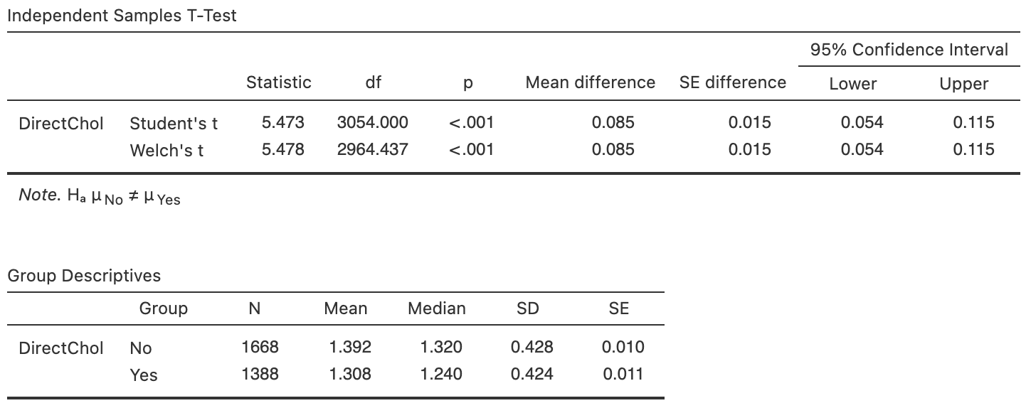
FIGURE 30.9: Software output for the nhanes data.

Exercise 30.7 Barrett et al. (2010) studied the effectiveness of echinacea to treat the common cold, and compared the mean duration of the cold for participants treated with echinacea or a placebo to determine if using echinacea reduced the mean duration of symptoms. Participants were blinded to the treatment, and allocated to the groups randomly. A summary of the data is given in Table 30.7.

1. What is the parameter? Carefully describe what it means.
2. Compute the standard error for the mean duration of symptoms for each group.
3. Compute the standard error for the difference between the means.
4. Sketch an error bar chart.
5. Compute an approximate \(95\)% CI for the difference between the mean durations for the two groups.
6. Compute an approximate \(95\)% CI for the population mean duration of symptoms for those treated with echinacea.
7. Write the hypotheses to answer the RQ.
8. Compute the standard error of the difference.
9. Compute the \(t\)-score, and approximate the \(P\)-value using the normal distribution tables.
10. Write a conclusion.
11. Are the CI and test statistically valid?
12. Are the results likely to be of practical importance?

TABLE 30.7: Numerical summary of duration (in days) of common cold symptoms, for blinded patients taking echinacea or a placebo.

	Mean	Standard deviation	Standard error	Sample size
Placebo	\(6.87\)	\(3.62\)		\(176\)
Echinacea	\(6.34\)	\(3.31\)		\(183\)
Difference	\(0.53\)

Exercise 30.8 Carpal tunnel syndrome (CTS) is pain experienced in the wrists. Schmid et al. (2012) compared two different treatments: night splinting, or gliding exercises.

Participants were randomly allocated to one of the two groups. Pain intensity (measured using a quantitative visual analogue scale; larger values mean greater pain) were recorded after one week of treatment. The data are summarised in Table 30.8.

1. What is the parameter? Carefully describe what it means.
2. In which direction is the difference computed? What does it mean when the difference is calculated in this way?
3. Compute the standard error for the mean pain intensity for each group.
4. Compute the standard error for the difference between the mean of the two groups.
5. Sketch an error bar chart.
6. Compute an approximate \(95\)% CI for the difference in the mean pain intensity for the treatments.
7. Compute an approximate \(95\)% CI for the population mean pain intensity for those treated with splinting.
8. Write the hypotheses to answer the RQ.
9. Compute the \(t\)-score, and approximate the \(P\)-value using the \(68\)--\(95\)--\(99.7\) rule.
10. Write a conclusion.
11. Are the CI and test statistically valid?

TABLE 30.8: Numerical summary of pain intensity for two different treatments of carpal tunnel syndrome.

	Mean	Standard deviation	Standard error	Sample size
Exercise	\(0.8\)	\(1.4\)		\(10\)
Splinting	\(1.1\)	\(1.1\)		\(10\)
Difference	\(0.3\)

Exercise 30.9 [Dataset: Dental] Woodward and Walker (1994) recorded the sugar consumption in industrialised (mean: \(41.8\,\text{kg}\)/person/year) and non-industrialised (mean: \(24.6\,\text{kg}\)/person/year) countries. The software output is shown in Fig. 30.10.

1. What is the parameter? Carefully describe what it means.
2. Write the hypotheses.
3. Using the software output (Fig. 30.10), write down and interpret the CI.
4. Write a conclusion for the hypothesis test.
5. Is the test statistically valid?

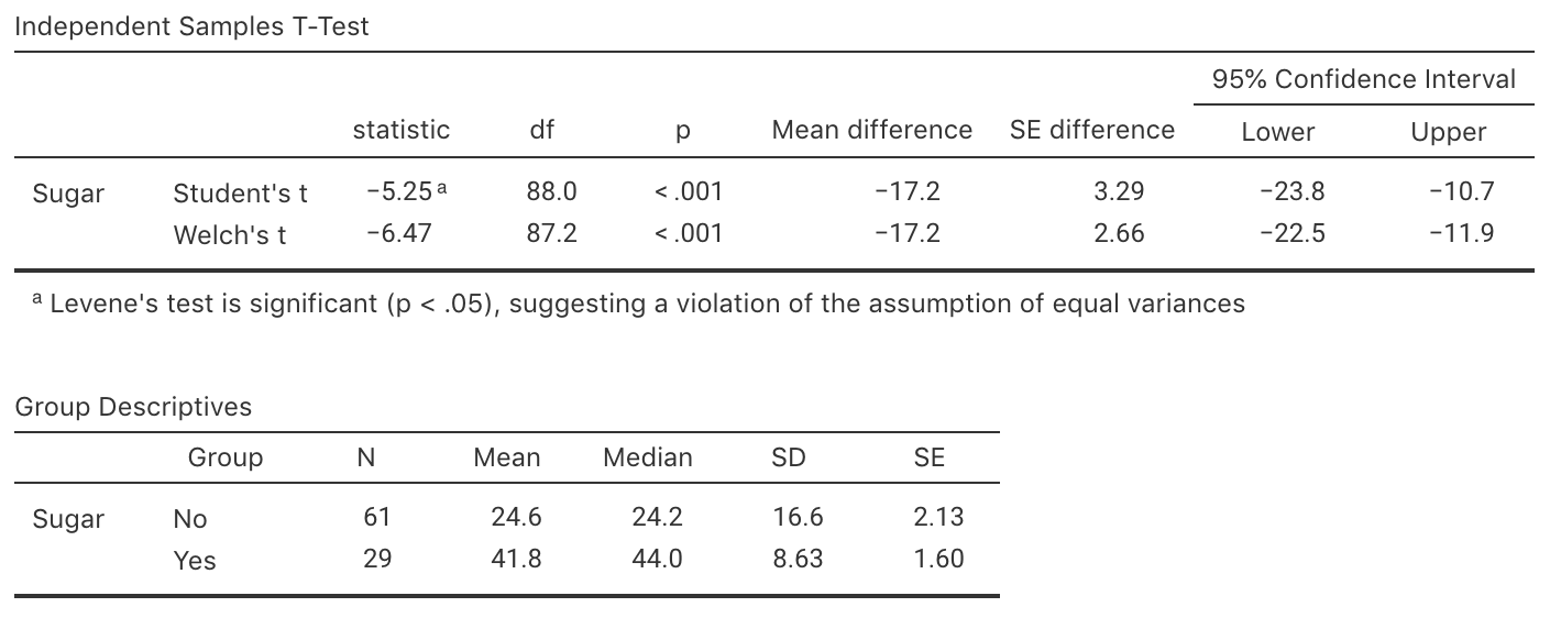
FIGURE 30.10: Software output for the sugar-consumption data; the Groups refer to whether or not the country is industrialised.

Exercise 30.10 [Dataset: Deceleration] To reduce vehicle speeds on freeway exit ramps, Ma et al. (2019) studied using additional signage. At one site studied (Ningxuan Freeway), speeds were recorded at various points on the freeway exit for vehicles before the extra signage was added, and then for different vehicles after the extra signage was added.

From this data, the deceleration of each vehicle was determined (Exercise 14.10) as the vehicle left the \(120\,\text{km}\).h^\(-1\) speed zone and approached the \(80\,\text{km}\).h^\(-1\) speed zone. Use the data, and the summary in Table 30.9, to test the RQ:

At this freeway exit, is the mean vehicle deceleration the same before extra signage is added and after extra signage is added?

Identify clearly the parameter of interest to understand how much the deceleration increased after adding the extra signage. Remember to compute and interpret the CI for this parameter.

TABLE 30.9: The signage deceleration data summary (in m.s\(^{-1}\)).

	Mean	Standard deviation	Standard error	Sample size
Before	\(\phantom{0}\phantom{0}0.0745\)	\(\phantom{0}0.0494\)	\(\phantom{0}0.00802\)	\(\phantom{0}38\)
After	\(\phantom{0}\phantom{0}0.0765\)	\(\phantom{0}0.0521\)	\(\phantom{0}0.00814\)	\(\phantom{0}41\)
Change	\(\phantom{0}{-0.0020}\)		\(\phantom{0}0.01143\)

Exercise 30.11 [Dataset: ForwardFall] A study (Wojcik et al. 1999) compared the lean-forward angle in younger and older women (Table 14.6). An elaborate set-up was constructed to measure this lean-forward angle, using harnesses. Consider this RQ:

Among healthy women, is the mean lean-forward angle greater for younger women compared to older women?

Use the software output (Fig. 30.11) to answer these questions:

1. What is the parameter? Carefully describe what it means.
2. What is an appropriate graph to display the data?
3. Construct an appropriate numerical summary from the software output (Fig. 14.10).
4. Construct approximate and exact \(95\)% CIs. Explain any differences.
5. Is the test one- or two-tailed?
6. Write the statistical hypothesis.
7. Use the software output to conduct the hypothesis test.
8. Write a conclusion.
9. Are the CI and test statistically valid?

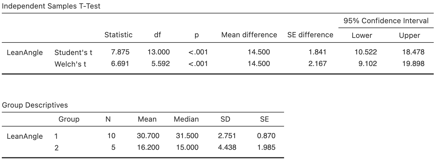
FIGURE 30.11: Software output for the face-plant data.

Exercise 30.12 Becker, Stuifbergen, and Sands (1991) compared the access to health promotion (HP) services for people with and without a disability in southwestern of the USA. 'Access' was measured using the quantitative Barriers to Health Promoting Activities for Disabled Persons (bhadp) scale. Higher scores mean greater barriers to health promotion services. The RQ is:

What is the difference between the mean bhadp scores, for people with and without a disability, in southwestern USA?

1. What is the parameter? Carefully describe what it means.
2. Sketch an error bar chart.
3. Compute the standard error of the difference.
4. Compile a numerical summary table.
5. Compute the approximate \(95\)% CI, and write a conclusion.
6. Write down the hypotheses.
7. Compute the \(t\)-score.
8. Determine the \(P\)-value.
9. Write a conclusion.
10. Are the CI and test statistically valid?

TABLE 30.10: The data summary for bhadp scores (no measurement units).

	Sample mean	Standard deviation	Sample size	Standard error
Disability	\(31.83\)	\(7.73\)	\(132\)	\(0.67280\)
No disability	\(25.07\)	\(4.80\)	\(137\)	\(0.41010\)
Difference	\(\phantom{0}6.76\)

Exercise 30.13 [Dataset: BodyTemp] Consider again the body temperature data from Sect. 27.1. The researchers also recorded the gender of the patients, as they also wanted to compare the mean internal body temperatures for females and males.

Use the software output in Fig. 30.12 to perform this test and to construct an approximate \(95\)% CI appropriate for answering the RQ. Comment on the practical significance of your results.

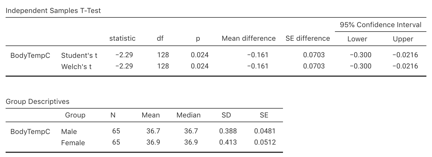
FIGURE 30.12: Software output for the body-temperature data.

Exercise 30.14 D. Chapman et al. (2007) compared 'conventional' male paramedics in Western Australia with male 'special-operations' paramedics. Some information comparing their physical profiles is shown in Table 30.11.

1. Compute the missing standard errors.
2. Compare the mean grip strength for the two groups of paramedics. (The standard error for the difference between the means is \(3.30\).)
3. Compare the mean number of push-ups completed in one minute for the two groups of paramedics. (The standard error for the difference between the means is \(4.0689\).)

TABLE 30.11: The physical profile of conventional (\(n = 18\)) and special operation (\(n = 11\)) paramedics in Western Australia.

	Conventional	Special Operations
Grip strength (in kg)
Mean	\(51\)	\(56\)
Standard deviation	\(\phantom{0}8\)	\(\phantom{0}9\)
Standard error
Push-ups (per minutes)
Mean	\(36\)	\(47\)
Standard deviation	\(10\)	\(11\)
Standard error

Exercise 30.15 [Dataset: Anorexia] Young girls (\(n = 29\)) with anorexia received cognitive behavioural treatment (Hand et al. (1996)), while another \(n = 26\) young girls received a control treatment (the 'standard' treatment). All girls had their weight recorded before and after treatment.

1. Determine the mean gain for individual girls using software.
2. Compute a CI for the mean weight gain for the girls in each group.
3. Compute a CI for the difference between the mean weight gains for the two treatment groups.
4. Conduct a test to determine if there is a difference between the mean weight gains for the two treatment groups.

Exercise 30.16 Researchers studied the impact of a gluten-free diet on dental cavities (Khalaf et al. 2020). Some summary information regarding the number decayed, missing and filled teeth (DMFT) is shown in Table 30.12. An exact \(95\)% CI is given as for the difference is \(-2.32\) to \(2.76\).

1. Using the \(68\)--\(95\)--\(99.7\) rule gives a slightly different CI. Why?
2. True or false: the difference is computed as the number of DMFT for coeliacs minus non-coeliacs.
3. True or false: one of the values for the CI is a negative value, which must be an error (as a negative number of DMFT is impossible).
4. We are \(95\)% confident that the difference between the population means is:

• Smaller for coeliacs;
• Between \(2.32\) higher for non-coeliacs to \(2.76\) higher for coeliacs.
• Between \(2.76\) higher for non-coeliacs to \(2.32\) higher for coeliacs.

TABLE 30.12: The summary of the number of DMFT for coeliacs and non-coeliacs.

	Sample size	Mean	Standard deviation	Standard error
Coeliacs	\(23\)	\(8.39\)	\(4.4\)	\(0.92\)
Non-coeliacs	\(23\)	\(8.17\)	\(4.1\)	\(0.86\)
Difference		\(0.22\)		\(1.30\)

Exercise 30.17 [Dataset: ReactionTime] Strayer and Johnston (2001) examined the reaction times, while driving, for students from the University of Utah (Agresti and Franklin 2007). In one study, students were randomly allocated to one of two groups: one group used a mobile phone while driving in a driving simulator, and one group did not use a mobile phone while driving in a driving simulator. The reaction time for each student was measured. The data are shown below.

Consider this RQ:

For students, what is the difference between the mean reaction time while driving when using a mobile phone and when not using a mobile phone?

---

Peter K. Dunn, 2024: CC BY-NC-SA 4.0