23 Confidence intervals: one mean
So far, you have learnt to ask a RQ, design a study, classify and summarise the data, and construct a confidence interval for one proportion. You have also been introduced to confidence intervals. In this chapter, you will learn to
- identify situations where estimating a mean is appropriate.
- form confidence intervals for one mean.
- determine whether the conditions for using the confidence intervals apply in a given situation.
23.1 Introduction
Consider rolling a fair, six-sided die \(n = 25\) times. Suppose we are interested in the mean of the numbers that are rolled. Since every face of the die is equally likely to appear on any one roll, the population mean of all possible rolls is \(\mu = 3.5\) (in the middle of the numbers on the faces of the die, so this is also the median).
What will be the sample mean of the numbers in the \(25\) rolls? We don't know, as the sample mean varies from sample to sample (sampling variation).
Remember: studying a sample leads to the following observations:
- Every sample is likely to be different.
- We observe just one of the many possible samples.
- Every sample is likely to yield a different value for the statistic.
- We observe just one of the many possible values for the statistic.
Since many values for the sample mean are possible, the values of the sample mean vary (called sampling variation) and have a distribution (called a sampling distribution).
23.2 Sampling distribution for \(\bar{x}\): for \(\sigma\) known
Suppose thousands of people made one sample of \(25\) rolls each, and computed the mean for their sample. Then, every person would have a sample mean for their sample, and we could produce a histogram of all these sample means (see the animation below). The mean for any single sample of \(n = 25\) rolls will sometimes be higher than \(\mu = 3.5\), and sometimes lower than \(\mu = 3.5\), but often close to \(3.5\).
From the animation above, the sample means vary with an approximate normal distribution (as with the sample proportions). This normal distribution does not describe the data; it describes how the values of the sample means vary across all possible samples. Under certain conditions (Sect. 23.5), the values of the sample mean vary with a normal distribution, and this normal distribution has a mean and a standard deviation.
The mean of this sampling distribution---the sampling mean---has the value \(\mu\). The standard deviation of this sampling distribution is called the standard error of the sample means, denoted \(\text{s.e.}(\bar{x})\). When the population standard deviation \(\sigma\) is known, the value of the standard error happens to be \[ \text{s.e.}(\bar{x}) = \frac{\sigma}{\sqrt{n}}. \] In summary, the values of the sample means have a sampling distribution described by:
- an approximate normal distribution,
- with a sampling mean whose value is \(\mu\), and
- a standard deviation, called the standard error, of \(\text{s.e.}(\bar{x}) = \sigma/\sqrt{n}\).
However, since the population standard deviation is rarely ever known, we will focus on the case where the value of \(\sigma\) is unknown (and estimated by the sample standard deviation, \(s\)).
23.3 Sampling distribution for \(\bar{x}\): for \(\sigma\) unknown
Since the value of the population standard deviation \(\sigma\) is almost never known, the sample standard deviation \(s\) is used to give an estimate of the standard error of the mean: \(\text{s.e.}(\bar{x}) = s/\sqrt{n}\). With this information, the sampling distribution of the sample mean can be described.
Definition 23.1 (Sampling distribution of a sample mean for the population standard deviation unknown) When the population standard deviation is unknown, the sampling distribution of the sample mean is (when certain conditions are met; Sect. 23.5) described by:
- an approximate normal distribution,
- centred around a sampling mean whose value is \(\mu\),
- with a standard deviation (called the standard error of the mean), denoted \(\text{s.e.}(\bar{x})\), whose value is \[\begin{equation} \text{s.e.}(\bar{x}) = \frac{s}{\sqrt{n}}, \tag{23.1} \end{equation}\] where \(n\) is the size of the sample, and \(s\) is the sample standard deviation of the observations.
A mean or a median may be appropriate for describing the data. However, the sampling distribution for the sample mean (under certain conditions) has a normal distribution. Hence, the mean is appropriate for describing the sampling distribution, even if not for describing the data.
23.4 Confidence intervals for \(\mu\)
In practice, we do not know the value of \(\mu\). After all, that's why we take a sample: to estimate the value of the unknown population mean. Suppose, then, we did not know the value of \(\mu\) for the die-rolling situation.
Then, we don't know the value of \(\mu\) (the parameter), but we have an estimate: the value of \(\bar{x}\), the sample mean (the statistic). The value of \(\bar{x}\) may be a bit smaller than \(\mu\), or a bit larger than \(\mu\) (but we don't know which, since we do not know the value of \(\mu\)). In other words, the values of \(\mu\) that may have produced the observed value \(\bar{x}\) may be less than the value of \(\bar{x}\), or greater than the value of \(\bar{x}\).
Since the values of \(\bar{x}\) vary from sample to sample (sampling variation) with an approximate normal distribution (Def. 23.1), the \(68\)--\(95\)--\(99.7\) rule could be used to construct an approximate \(95\)% interval for the plausible values of \(\mu\) that may have produced the observed values of the sample mean. This is a confidence interval.
A confidence interval (CI) for the population mean is an interval surrounding a sample mean. In general, a confidence interval for \(\mu\) is \[ \bar{x} \pm \overbrace{\big(\text{multiplier}\times\text{s.e.}(\bar{x})\big)}^{\text{The `margin of error'}}. \] For an approximate \(95\)% CI, the multiplier is about \(2\) (since about \(95\)% of values are within two standard deviations of the mean, from the \(68\)--\(95\)--\(99.7\) rule).
Definition 23.2 (Confidence interval for the population mean) A confidence interval (CI) for the unknown value of the population mean \(\mu\) is \[\begin{equation} \bar{x} \pm \big( \text{multiplier} \times \text{s.e.}(\bar{x})\big), \tag{23.2} \end{equation}\] where \(\big( \text{multiplier} \times \text{s.e.}(\hat{p})\big)\) is the margin of error, and \(\text{s.e.}(\bar{x})\) is the standard error of \(\bar{x}\) (see Eq. (23.1)), where \(\bar{x}\) is the sample mean, and \(n\) is the sample size. For an approximate \(95\)% CI, the multiplier is \(2\).
CIs are commonly \(95\)% CIs, but any level of confidence can be used (with the appropriate multiplier). In this book, a multiplier of \(2\) is used when approximate \(95\)% CIs are created manually, and otherwise software is used. Commonly, CIs are computed at \(90\)%, \(95\)% and \(99\)% confidence levels.
In Chap. 22, the multiplier was a \(z\)-score, and approximate values for the multiplier can be found using the \(68\)--\(95\)--\(99.7\) rule. When computing the CI for a sample mean, the multiplier is not a \(z\)-score (but is very similar to a \(z\)-score). The multiplier would be a \(z\)-score if the value of the population standard deviation was known (e.g., the situation in Sect. 23.2). When \(\sigma\) is unknown (almost always), and the sample standard deviation is used instead, the multiplier is a \(t\)-score (Sect. 27.4).
The values of \(t\)- and \(z\)-multipliers are very similar, and (except for small sample sizes) using an approximate multiplier of \(2\) is reasonable for computing approximate \(95\)% CIs in either case.
Pretend for the moment that the value of \(\mu\) was unknown, and we tossed a die \(25\) times, and found \(\bar{x} = 3.2\) and \(s = 2.5\). Then, \[ \text{s.e.}(\bar{x}) = \frac{s}{\sqrt{n}} = \frac{2.5}{\sqrt{25}} = 0.5. \] The sample means vary with an approximate normal distribution, centred around the unknown value of \(\mu\), with a standard deviation of \(\text{s.e.}(\bar{x}) = 0.5\) (Fig. 23.1).
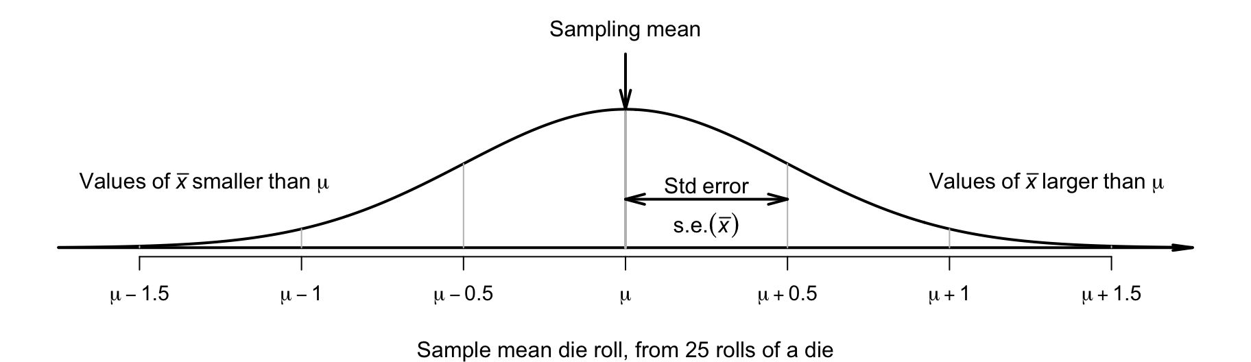
FIGURE 23.1: The sampling distribution is an approximate normal distribution; it shows a model of how the mean roll varies when a die is rolled \(25\) times.
Our estimate of \(\bar{x} = 3.2\) may be a bit smaller than the value of \(\mu\), or a bit larger than the value of \(\mu\); that is, the value of \(\mu\) is \(\bar{x}\) give-or-take a bit. A range of \(\mu\) values that are likely to straddle \(\bar{x}\) is given by a CI. An approximate \(95\)% CI is from \[\begin{align*} 3.2 - (2 \times 0.5) &\qquad\text{(which is $2.2$)}\\ \text{to}\quad 3.2 + (2 \times 0.5) &\qquad\text{(which is $4.2$)}. \end{align*}\] Hence, values of \(\mu\) between \(2.2\) to \(4.2\) could reasonably have produced a sample mean of \(\bar{x} = 3.2\).
Using software, the exact \(95\)% CI is from \(2.17\) to \(4.23\), the same as the approximate CI to one decimal place.
23.5 Statistical validity conditions
As with any confidence interval, the underlying mathematics requires certain conditions to be met so that the results are statistically valid (i.e., the sampling distribution is sufficiently like a normal distribution).
Statistical validity can be assessed using these criteria:
- When \(n \ge 25\), the test is statistically valid. (If the distribution of the data is highly skewed, the sample size may need to be larger.)
- When \(n < 25\), the test is statistically valid only if the data come from a population with a normal distribution.
The sample size of \(25\) is a rough figure, and some books give other values (such as \(30\)). For a CI for one mean, these conditions are the same as for the hypothesis test for one mean (Sect. 27.8).
This condition ensures that the sampling distribution of the sample means has an approximate normal distribution (so that, for example, the \(68\)--\(95\)--\(99.7\) rule can be used). Provided the sample size is larger than about \(25\), this will be approximately true even if the distribution of the individuals in the population do not have a normal distribution. That is, when \(n \ge 25\) the sample means generally have an approximate normal distribution, even if the data themselves do not follow a normal distribution. The units of analysis are also assumed to be independent (e.g., from a simple random sample).
If the statistical validity conditions are not met, other methods (e.g., non-parametric methods (Bauer 1972); resampling methods (Efron and Hastie 2021)) may be used.
When \(n \ge 25\) approximately, the data do not have to have a normal distribution. The sample means need to have a normal distribution, which is approximately true if the statistical validity conditions are true.
Example 23.1 (Statistical validity) In the die example (Sect. 23.4), where \(n = 25\), the CI is statistically valid.
The second statistical validity condition requires the population to have a normal distribution. Knowing this is obviously difficult; we do not have access to the whole population. All we can reasonably do is to identify (from the sample) whether the population is likely to be non-normal (when the CI would be not valid).

Example 23.2 (Statistical validity) A study (Silverman et al. 1999; Zou, Tuncali, and Silverman 2003) examine exposure to radiation for CT scans in the abdomen for \(n = 17\) patients. As the sample size is 'small' (less than \(25\)), the population data must have a normal distribution for a CI for \(\mu\) to be statistically valid.
A histogram of the total radiation dose received using the sample data (Fig. 23.2) suggests this is very unlikely. Even though the histogram is from sample data, it seems improbable that the data in the sample would have come from a population with a normal distribution.
A CI for the mean of these data will probably be not statistically valid. Other methods (such as resampling methods, which are beyond the scope of this book) are needed to compute a CI for the mean.
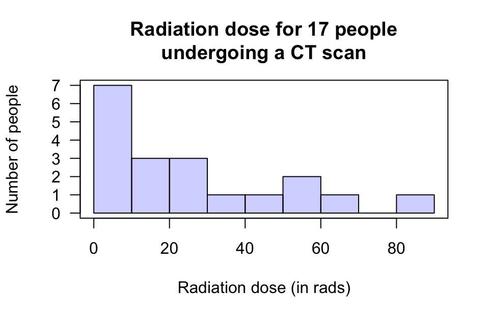
FIGURE 23.2: The radiation doses from CT scans for \(17\) people.
23.6 Example: cadmium in peanuts
Blair and Lamb (2017) studied peanuts gathered from a variety of regions in the United States over various times (a representative sample). They found the sample mean cadmium concentration was \(\bar{x} = 0.076\,\text{ppm}\) with a standard deviation of \(s = 0.0460\,\text{ppm}\), from a sample of \(290\) peanuts. The parameter is \(\mu\), the population mean cadmium concentration in peanuts.
Every sample of \(n = 290\) peanuts is likely to produce a different sample mean, so sampling variation in \(\bar{x}\) exists and can be measured using the standard error: \[ \text{s.e.}(\bar{x}) = \frac{s}{\sqrt{n}} = \frac{0.0460}{\sqrt{290}} = 0.002701\text{ ppm}. \] The approximate \(95\)% CI is \(0.0768 \pm (2 \times 0.002701)\), or \(0.0768 \pm 0.00540\), which is from \(0.0714\) to \(0.0822\,\text{ppm}\). (The margin of error is \(0.00540\).) We write:
The sample mean cadmium concentration of peanuts is \(\bar{x} = 0.0768\)(\(n = 290\)), with an approximate \(95\)% CI from \(0.0714\) to \(0.0822\).
If we repeatedly took samples of size \(290\) from this population, about \(95\)% of the \(95\)% CIs would contain the population mean (our CI may or may not contain the value of \(\mu\)). The plausible values of \(\mu\) that could have produced \(\bar{x} = 0.0768\) are between \(0.0714\) and \(0.0822\,\text{ppm}\). Alternatively, we are about \(95\)% confident that the CI of \(0.0714\) to \(0.0822\,\text{ppm}\) straddles the population mean.
Since the sample size is larger than \(25\), the CI is statistically valid.
23.7 Chapter summary
To compute a confidence interval (CI) for a mean, compute the sample mean, \(\bar{x}\), and identify the sample size \(n\). Then compute the standard error, which quantifies how much the value of \(\bar{x}\) varies across all possible samples: \[ \text{s.e.}(\bar{x}) = \frac{s}{\sqrt{n}}, \] where \(s\) is the sample standard deviation. The margin of error is (multiplier\({}\times{}\)standard error), where the multiplier is \(2\) for an approximate \(95\)% CI (from the \(68\)--\(95\)--\(99.7\) rule). Then the CI is: \[ \bar{x} \pm \left( \text{multiplier}\times\text{standard error} \right). \] The statistical validity conditions should also be checked.
23.8 Quick review questions
Are the following statements true or false?
- The value of \(\bar{x}\) varies from sample to sample.
- A CI for \(\mu\) is never statistically valid if the histogram of the data has a non-normal distribution.
- A sample of data produces \(s = 8\) and \(n = 20\); the standard error of the mean is \(1.7889\).
- Since the sample size is less than \(25\), the standard error is not statistically valid.
23.9 Exercises
Answers to odd-numbered exercises are given at the end of the book.
Exercise 23.1 Bartareau (2017) studied American black bears, and found the mean weight of the \(n = 185\) male bears was \(\bar{x} = 84.9\,\text{kg}\), with a standard deviation of \(s = 51.1\,\text{kg}\).
- Define the parameter of interest.
- Compute the standard error of the mean.
- Draw a picture of the approximate sampling distribution for \(\bar{x}\).
- Compute the approximate \(95\)% CI.
- Write a conclusion.
- Is the CI statistically valid?
Exercise 23.2 Dianat et al. (2014) studied the weight of the school bags of a sample of \(586\) children in Grades \(6\)--\(8\) in Tabriz, Iran. The mean weight was \(\bar{x} = 2.8\,\text{kg}\) with a standard deviation of \(s = 0.94\,\text{kg}\).
- Define the parameter of interest.
- Compute the standard error of the mean.
- Draw a picture of the approximate sampling distribution for \(\bar{x}\).
- Compute the approximate \(95\)% CI.
- Write a conclusion.
- Is the CI statistically valid?
Exercise 23.3 [Dataset: LungCap]
Tager et al. (1979) studied the lung capacity of children in East Boston.
They measured the forced expiratory volume (FEV) of a sample of \(n = 45\) eleven-year-old girls.
For these children, the mean lung capacity was \(\bar{x} = 2.85\) litres and the standard deviation was \(s = 0.43\) litres (Kahn 2005).
Find an approximate \(95\)% CI for the population mean lung capacity of eleven-year-old females from East Boston.
Exercise 23.4 Taylor et al. (2013) studied lead smelter emissions near children's public playgrounds. They found the mean lead concentration at one playground (Memorial Park, Port Pirie, in South Australia) was \(6\,956.41\) micrograms per square metre, with a standard deviation of \(7\,571.74\) micrograms of lead per square metre, from a sample of \(n = 58\) wipes taken over a seven-day period. (As a reference, the Western Australian Government recommends a maximum of \(400\) micrograms of lead per square metre.)
Find an approximate \(95\)% CI for the mean lead concentration at this playground. Would these results apply to playgrounds in other parts of Australia?
Exercise 23.5 Ian D. M. Macgregor and Rugg-Gunn (1985) studied the brushing time for \(60\) young adults (aged \(18\)--\(22\) years old), and found the mean tooth brushing time was \(33.0\,\text{s}\), with a standard deviation of \(12.0\,\text{s}\). Find an approximate \(95\)% CI for the mean brushing time for young adults.
Exercise 23.6 B. Williams and Boyle (2007) asked paramedics (\(n = 199\)) to estimate the amount of blood loss on four different surfaces. When the actual amount of blood spill on concrete was \(1\,000\,\text{mL}\), the mean guess was \(846.4\,\text{mL}\) (with a standard deviation of \(651.1\,\text{mL}\)).
- What is the approximate \(95\)% CI for the mean guess of blood loss?
- Do you think the participants are good at estimating the amount of blood loss on concrete?
- Is this CI statistically valid?
Exercise 23.7 [Dataset: NHANES]
Using data from the nhanes study (Control and (CDC) 1996), the approximate \(95\)% CI for the mean direct HDL cholesterol is \(1.356\) to \(1.374\,\text{mmol}\)/L.
Which (if any) of these interpretations are acceptable?
Explain why are the other interpretations are incorrect.
- In the sample, about \(95\)% of individuals have a direct HDL concentration between \(1.356\) to \(1.374\,\text{mmol}\)/L.
- In the population, about \(95\)% of individuals have a direct HDL concentration between \(1.356\) to \(1.374\,\text{mmol}\)/L.
- About \(95\)% of the samples are between \(1.356\) to \(1.374\,\text{mmol}\)/L.
- About \(95\)% of the populations are between \(1.356\) to \(1.374\,\text{mmol}\)/L.
- The population mean varies so that it is between \(1.356\) to \(1.374\,\text{mmol}\)/L about \(95\)% of the time.
- We are about \(95\)% sure that sample mean is between \(1.356\) to \(1.374\,\text{mmol}\)/L.
- It is plausible that the sample mean is between \(1.356\) to \(1.374\,\text{mmol}\)/L.
Exercise 23.8 Grabosky and Bassuk (2016) describe the diameter of Quercus bicolor trees planted in a lawn as having a mean of \(25.8\,\text{cm}\), with a standard error of \(0.64\,\text{cm}\), from a sample of \(19\) trees. Which (if any) of the following is correct?
- About \(95\)% of the trees in the sample will have a diameter between \(25.8 - (2\times 0.64)\) and \(25.8 + (2\times 0.64)\,\text{cm}\) (using the \(68\)--\(95\)--\(99.7\) rule).
- About \(95\)% of these types of trees in the population will have a diameter between \(25.8 - (2\times 0.64)\) and \(25.8 + (2\times 0.64)\,\text{cm}\) (using the \(68\)--\(95\)--\(99.7\) rule)?
Exercise 23.9 Watanabe et al. (1995) studied \(n = 30\) five-year-old children, and found the mean time for the children to eat a cookie was \(61.3\,\text{s}\), with a standard deviation of \(29.4\,\text{s}\).
- What is an approximate \(95\)% CI for the population mean time for a five-year-old child to eat a cookie?
- Is the CI statistically valid?
Exercise 23.10 [Dataset: PizzaSize]
In 2011, Eagle Boys Pizza ran a campaign that claimed (among many other claims) that Eagle Boys pizzas were 'Real size \(12\)-inch large pizzas' in an effort to out-market Domino's Pizza.
Eagle Boys made the data behind the campaign publicly available (P. K. Dunn 2012).
A summary of the diameters of a sample of \(125\) of Eagle Boys large pizzas is shown in Fig. 23.3.
What do \(\mu\) and \(\bar{x}\) represent in this context?
Write down the values of \(\mu\) and \(\bar{x}\).
Write down the values of \(\sigma\) and \(s\).
Compute the value of the standard error of the mean.
Explain the difference in meaning between \(s\) and \(\text{s.e.}(\bar{x})\) here.
If someone else takes a sample of \(125\) Eagle Boys pizzas, will the sample mean be \(11.486\) inches again (as in this sample)? Why or why not?
Draw a picture of the approximate sampling distribution for \(\bar{x}\).
Compute an approximate \(95\)% confidence interval for the mean pizza diameter.
Write a statement that communicates your \(95\)% CI for the mean pizza diameter.
What are the statistical validity conditions?
-
Which of these conditions must we assume are met for this CI to be statistically valid? Explain.
- The sample size is greater than about \(25\).
- The population has a normal distribution.
- The population standard deviation is known.
- The sample has a normal distribution.
Do you think that, on average, the pizzas do have a mean diameter of \(12\) inches in the population, as Eagle Boy's claim? Explain.
Exercise 23.11 Claire and Jake were wondering about the mean number of matches in a box. The boxes contain this statement:
An average of \(45\) matches per box.
They purchased a carton containing \(25\) boxes of matches, and Jake counted the number of matches in one of those \(25\) boxes. The box contained \(44\) matches.
'Oh wow. Just wow.' said Jake. 'They lie. There's only \(44\) in this box.'
What is Jake's misunderstanding?
-
Then, they counted the number of matches in each of the twenty-five boxes, and found the mean number of matches per box was \(44.9\) matches, and the standard deviation was \(0.124\).
Jake notes that the mean is \(44.9\) matches per box, and says: 'You can't have \(0.9\) of a match. That's dumb.' How would you respond?
-
'Wow!' said Jake. 'The claim is \(45\) matches per box on average, but the mean really is \(44.9\)! They're liars!'
What is Jake's misunderstanding?
What two broad reasons could explain why the sample mean is not \(45\)?
-
'Come on, Jake,' said Claire. 'As if the mean will be exactly \(45\) in a sample every single time. Let's work out the confidence interval.'
Why does Claire think a CI is needed? What will it tell them?
What is an approximate \(95\)% confidence interval for the mean for Claire's sample?
-
'Aha---I told you so! They are absolutely lying! Your confidence interval doesn't even include their mean of \(45\)!' said Jake. 'The manufacturer must be lying!'
Is Jake correct? Why or why not? What does the CI mean?
In this scenario, what does \(\bar{x}\) represent? What is the value of \(\bar{x}\)?
In this scenario, what does \(\mu\) represent? What is the value of \(\mu\)?
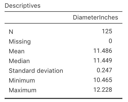
FIGURE 23.3: Summary statistics for the diameter of Eagle Boys large pizzas.