36 Reading and critiquing research

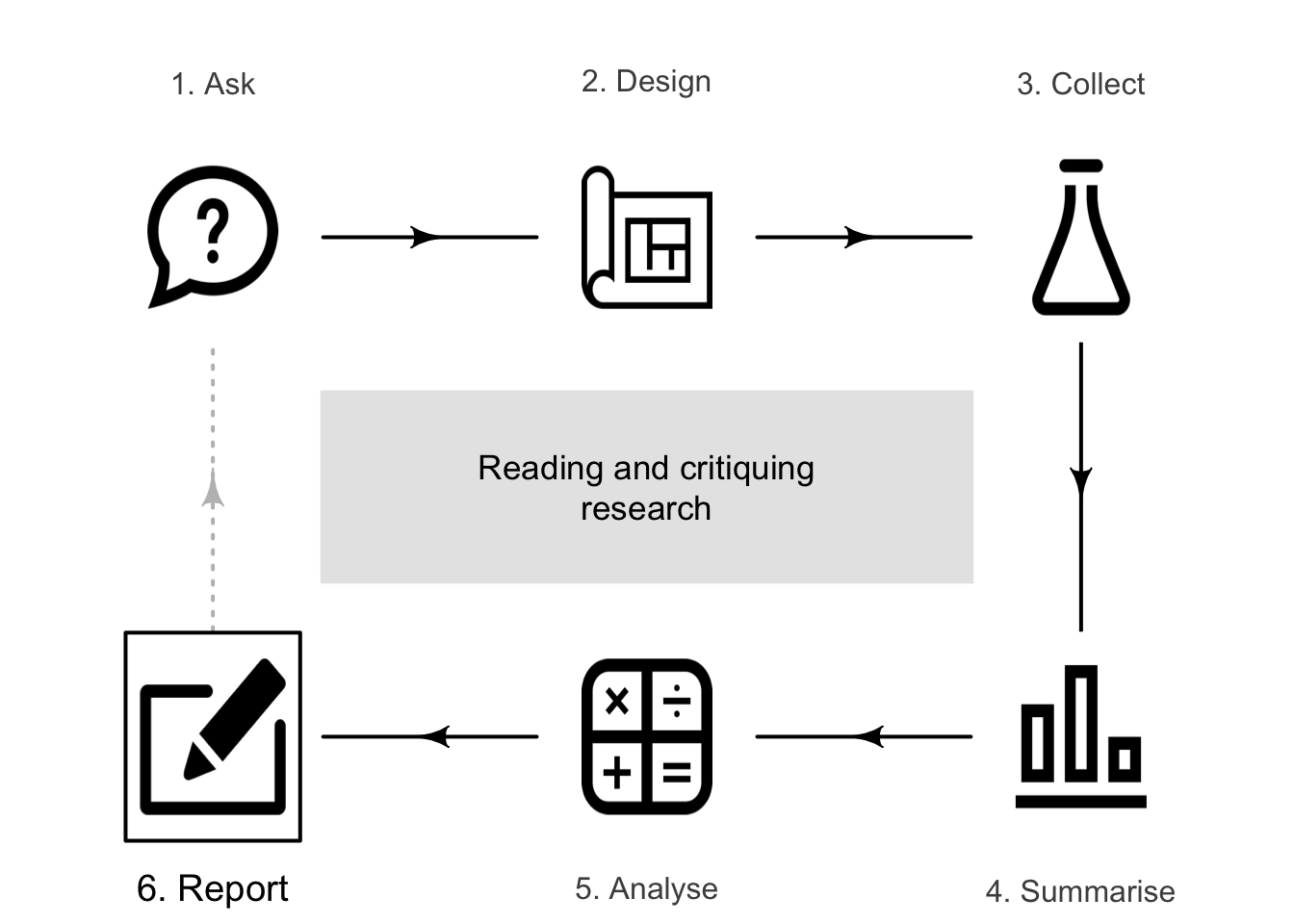
So far, you have learnt the about the process of research: asking a RQ, designing a study, collecting data, describing and summarising the data, and analysing the data (confidence intervals; hypothesis tests). You have learnt how to write about your research. In this chapter, you will learn to:

read and critique research.

36.1 Introduction

All academic disciplines change and adapt. Staying current in your discipline requires reading, critiquing and understanding the research of others, as communicated in journal articles or presentations (Chap. 35). (Critiquing means to evaluate: identifying what is good, and what can be improved.)

At some time during your studies or employment, you will need to read research articles:

to understand current practices in your discipline;
to know why your discipline uses the current procedures and practices;
to learn about new procedures and practices that may be adopted;
to critique the evidence for current or new practices; and
to identify open or unresolved questions in your discipline.

Familiarity with the language and concepts of research is important for understanding these articles, even if you will not be conducting your own research.

Reading research articles can be challenging. Rather than reading articles thoroughly from start to finish, first read the Abstract (Sect, 35.5.2)) to obtain an overview of the whole article, without becoming lost in the details. Then, read the Discussion, which highlights the important findings. Next, skim the rest of the article (perhaps focusing on graphs and tables of results). Finally, if necessary, read the article for details.

Terminology and notation varies widely in research (Sect. 35.6.3). When reading research, check the terminology and notation being used if you are unsure!

The six steps of the research process (Sect. 1.4) can guide the research critique.

Asking the RQ:

What research question is the research answering?
Why is this RQ important?
To what population will the results apply?
What are the units of analysis and units of observation?
How are important terms defined?

Designing the study:

Is the study observational or experimental?
Is the study well-designed? What is not explained or clear?
What design features and used, and why?
How many individuals are in the study?
How was the sample obtained? What are the implications for external validity?
Is the study designed to maximize internal validity?
How is confounding managed?
What are the design limitations?
Are there ethical concerns?
What is the source of funding?

Collecting the data:

How were the data collected?
Are the necessary details provided so the study can be approximately replicated?

Classifying and summarising the data:

Is the data summary appropriate, complete and clear?
What does the data summary reveal about the data?
What do the tables and graphs reveal about the data and relationships?

Analysing the data:

What types of confidence intervals and/or hypothesis tests were used?
Is the analysis appropriate, accurate, valid and clear?
What do the results mean?
What software was used?
Are the results statistically valid?

Reporting the results:

What are the main conclusions, and how do they answer the RQ?
Are the conclusion consistent with the results?
Are the results accurate, appropriate and well-reported?
Are the results of practical importance?
Are the study limitations acknowledged, and their implications discussed?
What other questions have emerged?

36.2 Example: walking while texting

Sajewicz and Dziuba-Słonina (2023) studied the impact of texting (using a smartphone) on how students walk. In this section, the article will be briefly discussed.

36.2.1 The Abstract

Part of the unstructured Abstract for the article reads:

The aim of this experiment was to investigate whether using a cell phone while walking affects walking velocity [...] in young people. Forty-two subjects ($20$ males, $22$ females; mean age: $20.74\pm 1.34$ years; mean height: $173.21\pm 8.07$ cm; mean weight: $69.05\pm 14.07$ kg) participated in the study. The subjects were asked to walk on an FDM--1.5 dynamometer platform four times at a constant comfortable velocity and a fast velocity of their choice. They were asked to continuously type one sentence on a cell phone while walking at the same velocity. The results showed that texting while walking led to a significant reduction in velocity compared to walking without the phone.

As this is the Abstract, many details are absent (but explained in the article itself). Nonetheless, a lot can be learnt about the study from the Abstract:

Asking the RQ:
This is a repeated-measures RQ: data are collected from the same students 'four times' (which are explained more fully in the article).
The population is 'young people'.
The numbers that follow the $\pm$ are not explained: are they confidence interval limits, standard deviations, IQRs, ranges, standard errors?
The units of analysis are the individual students in the study: each person has four measurements.
The main outcome is the (average) 'walking velocity'.
Designing the study:
The sampling method is not stated, but likely to be voluntary-response.
The sample size is $n = 42$.
Analyse the data:
A quantitative variable (walking velocity) is being compared within individuals, so paired $t$-tests are the likely method of analysis (Chap. 29).
Report the results:
Details of the analysis are not given (e.g., $P$-values or CIs).
Nonetheless, the conclusion is that 'walking led to a significant reduction in velocity compared to walking without the phone'.

36.2.2 Introduction

The Introduction introduces the context for the study, and establishes what is known about the topic. The aim of the study is (p. 1):

... to analyze how the use of a cell phone while walking at different velocities affects gait parameters, i.e., velocity, cadence, stride width, and stride length.

(Cadence refers to the tempo or rhythm of the walking, measure in steps per minute.)

36.2.3 Materials and Methods

The Material and Methods section provides details of the study, including:

The sample comprises students from the University School of Physical Education (Poland) studying a course in gait analysis. This sample may not represent any general population, though the conclusions may possibly apply to non-students and not-Poles.
Exclusion criteria (e.g., using lower limb prostheses) and inclusion criteria (e.g., daily use of a cell phone while walking) were given.
Extraneous variables collected included age, height, weight and sex.
The study was ethical, with permission sought from the students, and approval given by the Senate Committee on Research Ethics at the university.
Control variables included the temperature and humidity: 'the air temperature was constant at $22$ degrees Celsius, and the air humidity was $47$%' (p. 3).
Details of the specialised equipment used was given: 'The experiment was conducted using an FDM--1.5 Zebris dynamography platform'.
Further details of the protocol used were given.
Each subject participated in four tasks. In each, the subject (without footwear) made as many passes on the platform as possible in one minute:

The subject walked at a constant comfortable velocity (i.e., the velocity, chosen by the subject, that the person walks most naturally).
The subject walked at a constant fast velocity (i.e., as fast as the subject could comfortably walk, chosen by the subject).
Task 1 was repeated, with subjects continuously typing a sentence on a cell phone.
Task 2 was repeated, with subjects continuously typing a sentence on a cell phone.

Five response variables were used: left-side stride length, right-side stride length, cadence, stride width, and walking velocity. These appear to have been measured objectively.
The 'sentences' to be typed were defined as 'tongue twisters... not used in everyday conversation', but were not provided.
The analysis was given as 'paired Student’s $t$-test' in most cases, or the Wilcoxon test if the statistical validity conditions were not satisfied.
The software (and version) used was stated: TIBCO Statistica 13.3.0 (StatSoft Poland).

36.2.4 Results

The Results section provides the results of the analyses, including:

The data are not immediately available (probably due to ethics concerns) but 'are available upon request' (p. 7). Details of the analysis were not available.
Case-profile plots were produced for the five response variable, showing the means for each task rather than for all $42$ individuals (much like Fig. 13.2).
Correlations were computed between the five response variable. The correlations between stride width and the other variables were negative; all other correlations were positive. Since the relationship were non-linear, Spearman correlations were used rather than the Pearson correlations studied in Chap. 33. All the corresponding $P$-values were all less than $0.05$ apart from the correlation between stride width and cadence.
The following comparisons were made for each response variable:

Task 1 and Task 3 were compared: this explored the impact of texting on a smartphone when walking at a comfortable velocity.
Task 2 and Task 4 were compared: this explored the impact of texting on a smartphone when walking at a fast velocity.
Task 3 and Task 4 were compared: this explored the difference between texting and not texting when walking at a fast velocity.

The mean and standard deviation of the three response variables was provided for each task. However, the numerical summary for the differences were not provided; a $P$-value only was provided.
Fifteen hypothesis tests were conducted: the three between-tasks comparison listed above, for the five response variables.
The results are summarised as (p. 5):

... right and left single step length and gait velocity, were found to be statistically significant in each comparison. The value of the change in step width was statistically significant only when comparing trials 1 and 3, and cadence showed statistical significance when comparing trials 2 and 4, as well as 3 and 4.

'Statistically significant' was defined as a $P$-value smaller than $0.017$, rather than the commonly-used $P < 0.05$. The reason was to reduce the chance of making a Type I error (Sect. 28.7), but the details are beyond the scope of this book.
The researchers also made qualitative observations. For example: they observed 'moments when the subject took their eyes off the phone in order to assess the direction of the path' (p. 5).

36.2.5 Discussion

The Discussion includes the following statements:

The researchers concluded that 'the use of a cell phone while walking significantly affects gait parameters, causing a decrease in walking velocity and a reduction in stride length' (p. 6), thus providing answers to the RQs.
The researchers state (p. 6) that 'This proves that texting on a cell phone has a major impact on gait'. However, the research does not prove anything based on one of countless possible samples.
The researchers listed limitations of the study, including that the sentence typed by the subjects was unchanged in both Trials 3 and 4; hence, Trial 4 may have been easier than the previous trial as the sentence was familiar.
The researchers made recommendations: 'that the selection of the order of trials and the sentence to be typed on the cell phone be randomized' (p. 7).

36.3 Chapter summary

The six steps of research can be used as a scaffold for critiquing research articles. Starting by reading the Abstract (or Summary, or Overview) for an overview, then the Discussion, and then skim the rest of the article (perhaps focusing on graphs and tables of results). If necessary, read the article for details if needed.

36.4 Quick review questions

Are these statements true or false?

Reading an article thoroughly, from start to finish, is the best approach.
The six steps of research are a useful scaffold for critiquing an article.
Critiquing an article means to focus on finding all the problems.

36.5 Exercises

Answers to odd-numbered exercises are given at the end of the book.

Exercise 36.1 Duncan et al. (2018) examined the accuracy of step counts, as recorded on iPhones. The article states that participants

... were recruited through word of mouth and posters displayed around the [researcher's] university. Participants were eligible if they were ambulatory, $\ge 18$ years of age, and owned an iPhone 6 [...] or newer model.

How would you describe the sampling method? What is the implication?
How would you describe the information given about the subjects needing to be ambulatory and 18 years of age or over?

Although $33$ participants were selected, the authors note some parts of the study used a smaller sample size because one subject lost their phone, while others chose to withdraw from the study.

Why did the authors discuss these changes in sample size for some parts of the study?

The article notes that previous studies have been able to:

... demonstrate the accuracy of the iPhone pedometer function in laboratory test conditions. However, no studies have attempted to evaluate evidence [...] in the field.

Describe the issue that the authors raise with previous studies, using the language in this book.
Among many other things, the researchers compared the mean difference between the number of step counts recorded by manually counting steps (mean: $92.6$) and the iPhone-recorded number of steps (mean: $85.4$). What statistical test would be appropriate?
What hypotheses are being tested?
While walking at $2.5\,\text{km}$.h^$-1$, the above statistical test resulted in $t = 2.95$. What is the approximate $P$-value? Interpret the results.
The sample size for the analysis mentioned above was $n = 32$. Is the test statistically valid?

Exercise 36.2 Mohammadpoorasl et al. (2019) studied the relationship between hearing loss, and headphone and earphone use in Iranian students, using a non-directional study. The article states:

... $890$ students were randomly selected from five schools at qums [...] using a proportional cluster sampling method...

Only $866$ of the $890$ students agreed to participated in the study; of these, $745$ used earphones. The participants completed a hearing test and a Hearing Loss Questionnaire (HLQ; values between $17$ and $34$; higher scores indicating more severe hearing loss).

What is the population?
Is this an observational or experimental study?
Critique the sampling method. What is the implication for interpreting the results of the study?

One question in the HLQ is:

Does a hearing problem cause you difficulty when listening to TV or radio?

What is a potential problem with this question?
Compute the $95$% confidence interval for the proportion of students who had used earphones.

Some results are presented in Table 36.1.

What statistical test was appropriate for comparing the mean scores for males and females?
What are the hypotheses being tested?
What is the standard error for the difference between the means?
Perform the hypothesis tests; what do the results mean?
Compute the approximate $95$% confidence interval for the difference between the means.
Are the test and the CI statistically valid?

Table 36.1 also compares the HLQ scores for the frequency of earphone use specifically.

What are the hypotheses being tested?
Why is the sample size for this comparison only $791$ and not $845$?
Interpret the $P$-value for this test; what do the results mean?

Table 36.1 also compares the HLQ scores for those who use and do not use earphones.

Form an approximate $95$% CI for the mean hearing loss score for students who use earphones.
Compute the standard error of the difference between the mean hearing loss score for students who use and do earphones.
Perform a hypothesis test to compare the difference between the mean hearing loss score for students who use and do not use earphones, and confirm that the $P$-value is indeed very small.

TABLE 36.1: The Hearing Loss Questionnaire scores for various demographic variables.
		HLQ
Levels	Sample size	Mean	Std dev.	$P$-value
Sex
Female	$543$	$19.37$	$2.91$	$0.009$
Male	$302$	$19.99$	$3.51$
Frequency of earphone use
$0$, $1$ times/day	$194$	$19.20$	$2.87$	$0.001$
$2$ to $3$ times/day	$319$	$19.60$	$2.66$
More than $3$ times/day	$278$	$20.20$	$3.54$
Earphone use
Yes	$745$	$19.80$	$3.08$	less than $0.001$
No	$100$	$19.00$	$1.71$

Exercise 36.3 Mesrkanlou et al. (2023) studied the effect of an earthquake on pregnant mothers in Varzaghan, Iran (p. 2), using:

... $1000$ cases of pregnant women living in urban and rural areas of Varzaghan city that consisted of $550$ pre-earthquake and $450$ post-earthquake cases.

The researchers compared the mothers in the two groups (pre- and post-earthquake) on various measurements. For example, the mean age of mothers in the pre-group was $25.82$ y, and the mean age of the mothers in the post-group was $26.71$ y; the difference has a $P$-value of $0.084$.

What does this result mean?
Why did the researchers make this comparison between the mothers' ages in two groups?
What type of hypothesis test was used to make this conclusion?

The researchers also compared the mean birth weights of the babies born to the mothers in the two groups. In the pre-group, the mean birth weight was $3.25\,\text{kg}$ ($s = 0.52$) and in the post-group the mean birth weight was $3.18\,\text{kg}$ ($s = 0.54$).

Compute the standard error for comparing the difference between the two means.
Perform a hypothesis test to compare the mean birthweights. Interpret the results.
The two-tailed $P$-value for this test as given as $0.001$. Is this consistent with your calculations?

The researchers also compared the percentage of babies with a Low Birth Weight (LBW; less than $2.5\,\text{kg}$). For the pre-group, the percentage was $6.01$%; for the post-group, the percentage was $8.92$%.

What type of definition is given for LBW?
Construct the $2\times 2$ table for displaying these data.
What type of test was probably used for this comparison?
For the test, $\chi^2 = 3.052$. Deduce the equivalent $z$-score and the approximate $P$-value.
What limitations can you identify for this study?

Exercise 36.4 Tracy, Oster, and Beaver (1990) studied the selenium (Se) concentration in irrigation and stock water sources in California. For drinking water, the maximum recommended concentration was $10$ $\mu$g.L^$-1$; for irrigation water, the maximum recommended concentration was $20$ $\mu$g.L^$-1$

Part of the study examined the area within $5\,\text{km}$ of wells. When Pliocene rocks were within this radius, the relationship between the Se concentration $y$ in the water and the electrical conductivity of the water $x$ (in deciSiemens per meter, dS.m^$-1$) was $\hat{y} = -3.1 + 7.0x$, where $R^2 = 27$%.

Interpret the meaning of $R^2$.
What is the value of the correlation coefficient?
The $P$-value for testing the slope is $P < 0.001$. Interpret what this means in this context.
What are the measurement units of the slope?

For the $n = 151$ wells in the study, Table 36.2 shows the selenium concentration of the water and the geology within $5\,\text{km}$ of the well.

What hypotheses are being tested by the table?
The article states that $\chi^2 = 31.5$. What is the equivalent $z$-score for the test?
What is the approximate $P$-value for the test? Interpret what this means.

TABLE 36.2: Number of wells with dissolved Se above $2$ $\mu$g.L$^{-1}$, and the geology within $5$radius of the well.
	No	Yes
Se concentration $\le 2$ $\mu$g.L$^{-1}$	$78$	$15$
Se concentration greater than $2$ $\mu$g.L$^{-1}$	$23$	$35$

Exercise 36.5 M. C. Russell (2023) compared the larvae of two types of mosquitoes: Ae. albopictus (an invasive specie) and Cx. pipiens (a native species). One study compared the survival rates of the larvae at two temperatures (p. 4). At $15$^oC and $25$^oC, the survival rates were $86.8$% and $86.1$%, respectively. The papers states that these survival rates 'did not differ significantly', and quoted a $P$-value of $P = 0.8076$.

What type of test was probably used?
Interpret what the $P$-value means in this context.

The researchers also compared the size of the surviving larvae (p. 4 and 5) in the two control groups, using a two sample $t$-test. They found that control larvae were 'significantly larger' for Cx. pipiens compared to Ae. albopictus larvae. The paper then gives this information:

$\text{mean}\pm\text{SD}$: Cx. pipiens${} = 1.64 \pm 0.18\,\text{mm}$, Ae. albopictus${} = 1.36 \pm 0.13\,\text{mm}$; $\text{$p$-value} =< .0001$.

The two sample sizes are $n = 410$ and $n = 498$ respectively.

How would these results be interpreted?
What type of test would probably have been used?
Compute the standard error for the difference between the two types of mosquitoes.
Compute the $t$-score and approximate $P$-value for the test. What does the mean?
Is the $P$-value in the article consistent with your calculations?
Is the test statistically valid?

The length of the surviving larvae from both species were compared for the two temperatures also (p. 5): For surviving Cx. pipiens, control larvae were larger at $15$^oC compared to $25$^oC. The paper reports:

$\text{mean} \pm \text{SD}$: $15$^oC ${}= 1.66 \pm 0.01\,\text{mm}$, $25$^oC ${} = 1.60 \pm 0.02\,\text{mm}$; $\text{$p$-value} = .0065$.

For surviving Ae. albopictus, control larvae were larger at $15$^oC compared to $25$^oC. The paper reports:

$\text{mean} \pm \text{SD}$: $15$^oC ${}= 1.66 \pm 0.01\,\text{mm}$, $25$^oC ${} = 1.60 \pm 0.02\,\text{mm}$; $\text{$p$-value} = .0065$.

How would these results be interpreted?
What type of test would probably have been used?

Megacyclops viridis (a copepod) preys on the larvae. The linear association between predation efficiency ($y$; as a percentage) and predator--prey size-ratio ($x$; no units) was found (using $n = 45$) to be $\hat{y} = -19.56 + 31.64x$. The standard errors of the two regression coefficients were $17.92$ (intercept) and $13.88$ (slope).

Find an approximate $95$% confidence interval for each regression parameter.
Estimate the $P$-value for testing if the population slope is zero. Interpret what this means.
Is this test statistically valid?
Interpret the meaning of the slope.
The value of $R^2$ was given as $0.087$ (i.e., $8.7$%). Interpret this value.
Find the value of the correlation coefficient, $r$.

Exercise 36.6 Li, Jia, and Zhang (2017) studied the maximum mouth opening (MMO; in mm) for $452$ Chinese adults aged from $20$ to $35$.

Would the individuals in the study have been blinded? Explain. What are the implications?

The correlation between height and MMO was given as $r = 0.54$ with $P < 0.001$.

What does this mean?
Compute and interpret the value of $R^2$.

The regression equation relating the height $x$ (in cm) and MMO $y$ was given as $\hat{y} = 0.36x - 10.15$.

Interpret the estimates of the regression parameters.
Use the regression equation to predict the MMO for a person $179\,\text{cm}$ tall.

The mean MMO of males was $54.18\,\text{mm}$ ($s = 5.21$), and for females was $49.62\,\text{mm}$ ($s = 3.69$).

What type of hypothesis tests was used to compare the mean MMO for males and females?
The $t$-score for comparing MMO for males and females is $t = 10.63$. What is the $P$-value?
Is this result statistically valid?
What is the meaning of this comparison?
Is gender likely to be a confounding variable in this regression analysis? Explain carefully.

The authors state one of the limitations as:

First, participants were recruited from a pool of people who were undergoing regular medical examinations in our hospital [...]

What does this mean? What are the implications? Are there other limitations?

Exercise 36.7 Drinkwater et al. (1995) compared tomatoes growing on conventional (CNV; $n = 14$) and organic (ORG; $n = 17$) farms. Between 1989 and 1990, the researchers sampled tomato fields during April and September (p. $1\,100$). An area between $0.04$ and $0.1\,\text{ha}$ was set aside within each field for collecting data. Each area was divided into $20$ sections then, a $1\,\text{m}$ row was selected at random within each section to be sampled.

Explain what type of sampling is being used.

One important measure of soil health is the number of actinomycetes. When comparing ORG and CNV, the researchers found that the (p. $1\,103$):

... total numbers of actinomycetes [...] were significantly larger in the ORG soils [...] (Student's $t$ test, $t = 5.4$, $P = 0.006$)...

What type of test would probably have been used to reach this conclusion?
Explain what the results mean.
Are the results statistically valid?

The researchers also found that (p. $1\,103$):

... starch hydrolyzing actinomycetes were more numerous in CNV [...] (Student's $t$ test, $t = 4.0$, $P = 0.005$).

What type of test would probably have been used to reach this conclusion?
Explain what these results mean.

They also found that (p. $1\,103$):

Total actinomycete abundance [was] negatively correlated with corky root [a disease] severity ($r = -0.76$, $P = 0.08$;...).

Explain what these results mean.
Compute and interpret the value of $R^2$.

Exercise 36.8 Teo et al. (2022) studied pregnant Malaysian women with sleeping disruptions in the last month of pregnancy. The $56$ patients were (p. 1):

... randomized to the use of eye-mask and earplugs or "sham" headbands during night sleep (both introduced as sleep aids).

Thus, two groups were used: one using eye-masks and earplugs (treatment group, T; $n = 29$) and one using sham headbands (control or placebo group, P; $n = 27$).

What was the purpose of using 'sham' headbands if it was an ineffective intervention?
What type of study is this: experimental or observational? Explain.

Sleep duration was measured in Week 1 (no intervention) and again in Week 2 (with the allocated intervention) for each subject, using a 'wrist actigraphy monitor'.

Why is using a 'wrist actigraphy monitor' better than self-reported sleep duration?

The women in the two groups were compared. For example, the mean age of the women was $30.6$ y ($s = 3.6$) (T) and $30.1$ y ($s = 3.3$) (P); the $P$-value for the comparison was given as $P = 0.56$.

Why was this comparison made?
Compute the standard error for the difference between the two mean sleep durations.
Compute the $t$-score for the test.
Is the quoted $P$-value consistent with your calculations? What do these results mean?
Is the result statistically valid?

Another comparison was the room 'condition' where the women slept: in the treatment group, $13$ had a room with a fan ($16$ had air conditioning), while in the control group $10$ women had a fan (and $17$ air conditioning). The $P$-value for the comparison was given as $P = 0.60$.

Why was this comparison made?
Construct the $2\times 2$ table summarising the data.
The $\chi^2$-score for the test is $0.35064$. Compute the equivalent $z$-score. Interpret the results.
Is the quoted $P$-value consistent with your calculations?
Is the result statistically valid?

In the treatment group, the mean sleep duration in Week 1 was $279.0\,\text{mins}$ ($s = 18.9$) and in Week 2 was $303.6\,\text{mins}$ ($s = 18.8$). The increase was $24.7\,\text{mins}$ ($s = 14.9$).

Test if sleep duration increased in the treatment group. Interpret the results mean.

In the control group, the mean sleep duration in Week 1 was $286.3\,\text{mins}$ ($s = 20.9$) and in Week 2 was $301.9\,\text{mins}$ ($s = 21.8$; $n = 26$). The increase was $18.1\,\text{mins}$ ($s = 17.3$).

Test if sleep duration increased in the control group. Interpret the results.
Why would sleep duration increase, if the control group used an ineffective intervention?

The increase in sleep duration can be compared for the two groups.

Compute the standard error for difference between the mean increases $\text{s.e.}( \bar{x}_T - \bar{x}_T)$.
Compare the increase in sleep duration for the two groups. Interpret the results.
Is the test statistically valid?

35 Reporting and writing research

A Datasets

		HLQ
Levels	Sample size	Mean	Std dev.	\(P\)-value
Sex
Female	\(543\)	\(19.37\)	\(2.91\)	\(0.009\)
Male	\(302\)	\(19.99\)	\(3.51\)
Frequency of earphone use
\(0\), \(1\) times/day	\(194\)	\(19.20\)	\(2.87\)	\(0.001\)
\(2\) to \(3\) times/day	\(319\)	\(19.60\)	\(2.66\)
More than \(3\) times/day	\(278\)	\(20.20\)	\(3.54\)
Earphone use
Yes	\(745\)	\(19.80\)	\(3.08\)	less than \(0.001\)
No	\(100\)	\(19.00\)	\(1.71\)

	No	Yes
Se concentration \(\le 2\) \(\mu\)g.L\(^{-1}\)	\(78\)	\(15\)
Se concentration greater than \(2\) \(\mu\)g.L\(^{-1}\)	\(23\)	\(35\)