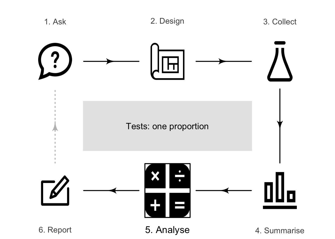
26 Hypothesis tests: one proportion

So far, you have learnt to ask a RQ, design a study, classify and summarise the data, and form confidence intervals. In this chapter, you will learn to:

• identify situations where conducting a test for a proportion is appropriate.
• conduct hypothesis tests for one sample proportion, using a \(z\)-test.
• determine whether the conditions for using these methods apply in a given situation.

26.1 Introduction: rolling dice

When in a toy store one day (for my children, of course), I saw 'loaded dice' for sale. The packaging claimed one loaded & one normal. I bought two sets! However, there was no indication as to which die was the loaded die. How could I determine which of the dice was loaded? That is, how could I make a decision about which die was loaded?

For a die that is not loaded, the population proportion of rolling any face of the die is \(p = 1/6\). So, for example, the population proportion of rolls that show a ⚀ is \(p = 1/6\), using the classical approach to probability. In any sample of rolls, however, the proportion of rolls showing a ⚀ would vary due to sampling variation, but would be approximately \(\hat{p} = 1/6\) with a fair die.

Suppose I rolled one die a certain number of times (say, \(n = 50\) times), then determined the value of the sample proportion. The sample proportion of rolls that show a ⚀ is unlikely to be exactly \(1/6\) (the population proportion). If the observed value of \(\hat{p}\) was not exactly \(1/6\), two possible reasons could explain this discrepancy:

• I was rolling the fair die (with \(p = 1/6\)), and the discrepancy between the population and sample proportions was simply due to sampling variation.
• I was rolling the loaded die (with \(p \ne 1/6\)), and the discrepancy between the population and sample proportion simply reflected this.

If I observed an unusually small or unusually large sample proportion of rolls that showed a ⚀, I would suspect that I had the loaded die: I was observing something unusual from a fair die. This is exactly the decision-making process seen in Chap. 25.

More formally then, the decision-making process (Chap. 25) could proceed as follows:

• Make an assumption about the parameter (Sect. 25.4.1): assume I have a fair die, so that \(p = 1/6\), where \(p\) is the population proportion of rolls that show a ⚀.
• Describe the expectations of the statistic (Sect. 25.4.2): describe what value of the sample proportion \(\hat{p}\) could reasonably be expected from a fair die.
• Take the sample observations (Sect. 25.4.3): roll the die many times to find a value of \(\hat{p}\).
• Make a decision (Sect. 25.4.4) based on what is observed in the sample.

Using this decision-making process (Fig. 26.1), I could decide if the die I had rolled seemed to be the fair die. For one specific die, I am asking the decision-making RQ:

For this die, is the population proportion of rolls that show a ⚀ equal to \(1/6\)?

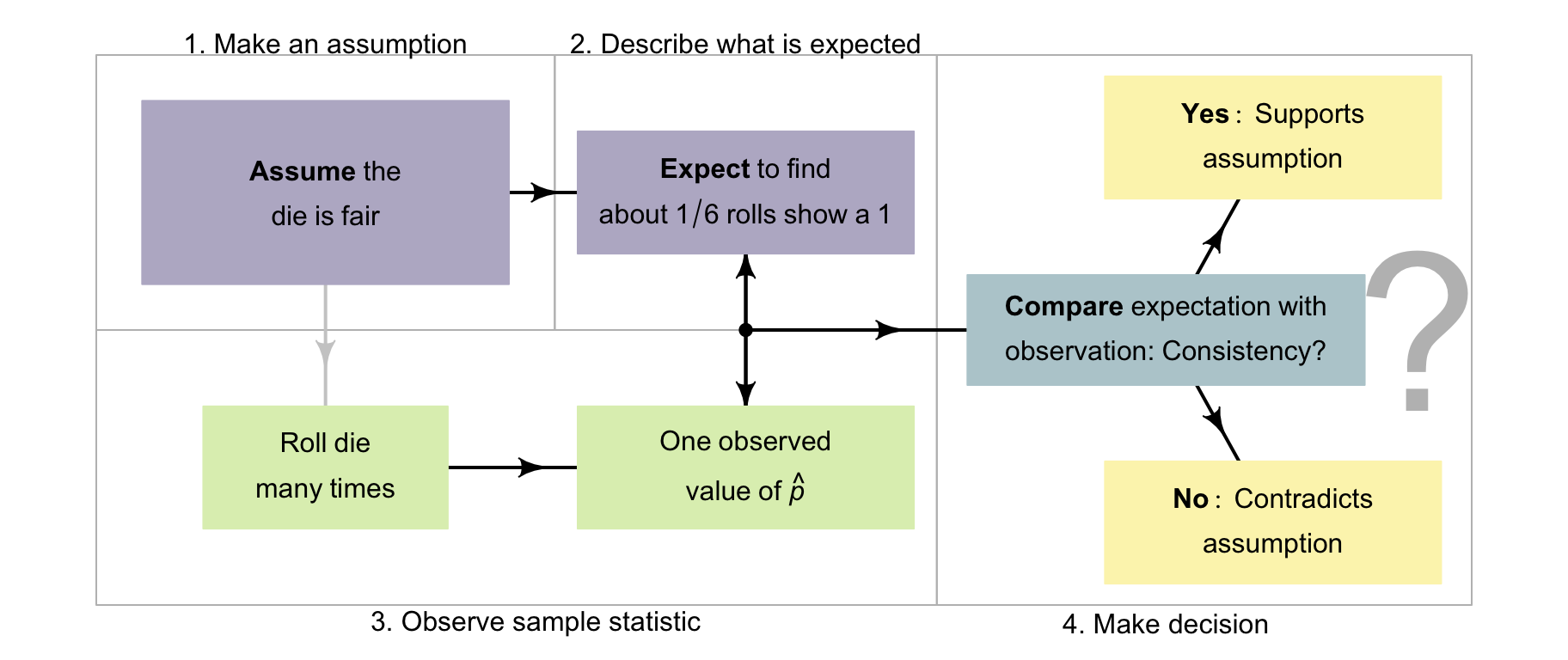
FIGURE 26.1: A way to make decisions for the dice example.

Answering a decision-making RQ such as this requires a hypothesis test. The process requires being able to describe what value of the sample proportion \(\hat{p}\) could reasonably be expected from a fair die, with \(p = 1/6\) (that is, Step 3 of the decision-making process).

\(p\) refers to the population proportion, and \(\hat{p}\) refers to a sample proportion.

26.2 Rolling dice: the sampling distribution of \(\hat{p}\)

When a fair, six-sided die is rolled \(50\) times, what proportion of the rolls will produce a ⚀? That is, what will be the value of the sample proportion \(\hat{p}\)? Of course, no-one knows, because the sample proportion will not be the same for every sample of \(50\) rolls. The sample proportion varies from sample to sample: sampling variation exists and is described by the sampling distribution.

As seen in Chap. 19, the sample statistic often varies with a normal distribution (whose standard deviation is called the standard error). However, being more specific about the details of this sampling distribution (i.e., the mean and standard deviation describing the normal model) is useful.

Remember: studying a sample leads to the following observations:

• Every sample is likely to be different.
• We observe just one of the many possible samples.
• Every sample is likely to yield a different value for the statistic.
• We observe just one of the many possible values for the statistic.

Since many values for the sample proportion are possible, the values of the sample proportion vary (called sampling variation) and have a distribution (called a sampling distribution).

To better understand the sampling distribution for the proportion of rolls that show a ⚀ in \(50\) rolls of a die, statistical theory could be used, or thousands of repetitions of a sample of \(50\) rolls could be performed, or a computer could simulate many samples of \(50\) rolls (as for a roulette wheel in Sect. 19.2).

Here, the population proportion of rolls showing a ⚀ is \(p = 1/6\) (using the classical approach to probability). Each sample of \(n = 50\) rolls produces a sample proportion, denoted by \(\hat{p}\), which varies from sample to sample.

These sample proportions would be expected to vary around \(p = 1/6\) (the population proportion): some values of \(\hat{p}\) would be larger than \(p\) and some smaller than \(p\). The value of the sample proportion in \(50\) rolls could be very small or very high by chance, but we wouldn't expect to see that very often. The sample proportions exhibit sampling variation, and the amount of sampling variation is quantified using a standard error.

Suppose a fair die was rolled \(50\) times, and this random procedure was repeated thousands of times, and the proportion of rolls that showed a ⚀ was recorded for every one of those thousands of sets of \(50\) rolls. These thousands of sample proportions \(\hat{p}\) (one from every sample of \(n = 50\) rolls) could be shown using a histogram; see the animation below.

In fact, the sampling distribution of \(\hat{p}\) was described in Def. 22.1 (and repeated in Def. 26.1). The sample proportions are described by

• an approximate normal distribution,
• centred around the sampling mean, with a value of \(p = 1/6\),
• with a standard deviation, called the standard error \(\text{s.e.}(\hat{p})\), of \[\begin{equation} \text{s.e.}(\hat{p}) = \sqrt{ \frac{p\times(1 - p)}{n} } = \sqrt{ \frac{1/6\times(1 - 1/6)}{50} } = 0.0527. \tag{26.1} \end{equation}\]

Definition 26.1 (Sampling distribution of a sample proportion with the population proportion known) For a known value of \(p\), the sampling distribution of the sample proportion is (when certain conditions are met; Sect. 22.7) described by

• an approximate normal distribution,
• centred around the sampling mean whose value is \(p\),
• with a standard deviation (called the standard error of \(\hat{p}\)), denoted \(\text{s.e.}(\hat{p})\), whose value is \[\begin{equation} \text{s.e.}(\hat{p}) = \sqrt{\frac{ p \times (1 - p)}{n}}, \tag{26.2} \end{equation}\] where \(n\) is the size of the sample used to compute \(\hat{p}\), and \(p\) is the population proportion.

A picture of this normal distribution can be drawn (Fig. 26.2). The standard error is the standard deviation of the normal distribution in Fig. 26.2. While we still don't know exactly what values of \(\hat{p}\) the next set of \(50\) rolls will produce, we have some idea of how the sample proportion varies in samples of \(50\) rolls. For instance, values of \(\hat{p}\) greater than about \(0.35\) are unlikely to be observed from a fair die (with \(p = 1/6\)).

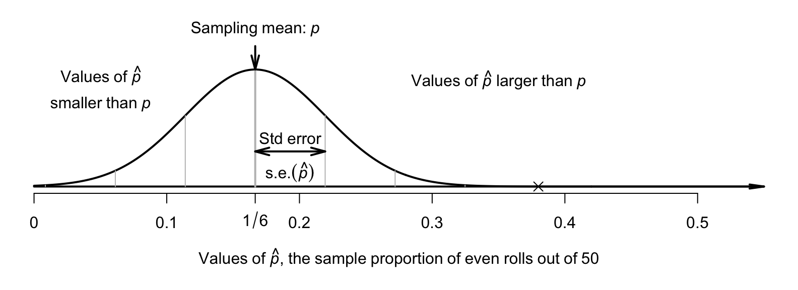
FIGURE 26.2: The sampling distribution is an approximate normal distribution; it shows a model of how the proportion of rolls showing a ⚀ varies, when a die is rolled \(50\) times. The cross represents the observed sample proportion.

26.3 Rolling dice: making a decision

Figure 26.2 show what values of the sample proportion \(\hat{p}\) are expected when a fair die is rolled. Step 3 of the decision-making process (Fig. 26.1) is to now roll the die.

When I rolled the die, a ⚀ appeared \(19\) times in my \(50\) rolls, a sample proportion of \[ \hat{p} = \frac{19}{50} = 0.38. \] In this unusual or unexpected? Locating this value of \(\hat{p}\) on the sampling distribution in Fig. 26.2 shows that a sample proportion of \(\hat{p} = 0.38\) is highly unusual from a fair die with \(p = 1/6\). More specifically, since the sampling distribution has a normal distribution, the \(z\)-score is \[ z = \frac{\text{statistic} - \text{mean of the distribution}}{\text{std dev. of the distribution}} = \frac{0.38 - (1/6)}{0.05270} = 4.05, \] which is a very large \(z\)-score (based on the \(68\)--\(95\)--\(99.7\) rule). Using a fair die, observing \(\hat{p} = 0.38\) would almost never occur. But I did observe \(\hat{p} = 0.38\), which suggests that the die I was rolling was not the fair die.

I concluded that the die I was rolling was loaded (that is, \(p \ne 1/6\)). I may be incorrect (after all, it is not impossible to observe \(\hat{p} = 0.38\)), but the evidence is certainly convincing. Using the decision-making process, a decision has been made about the dice.

The process described above is called hypothesis testing. Hypothesis testing is used to make decisions about a population after observing just one of the countless possible samples. Formally, the hypothesis test above proceeds as described in the following sections.

26.4 The process of hypotheses testing: assumption

Step 1 in the decision-making process is to make an assumption about the parameter. For the die example, the parameter is \(p\), the population proportion of rolls that show a ⚀. The assumption is that \(p = 1/6\). This is called the null hypothesis, denoted by \(H_0\): \[ \text{$H_0$: } p = 1/6. \] The null hypothesis states the value of \(p\) is \(1/6\); in other words, if the sample proportion \(\hat{p}\) is not equal to \(1/6\), the discrepancy is explained by sampling variation. The null hypothesis is always the 'sampling variation' explanation for the discrepancy between the values of the statistic and the parameter.

The other explanation for why the value of the sample proportion \(\hat{p}\) is not equal to \(1/6\) is called the alternative hypothesis (denoted \(H_1\)): that the population proportion is not \(1/6\), and this is the cause of the discrepancy: \[ \text{$H_1$: } p \ne 1/6. \] These two hypotheses offer different explanations for the discrepancy between the values of the population proportion (the parameter) and the sample proportion (the statistic). The null hypothesis \(H_0\) states that \(p = 1/6\) and the discrepancy is due to sampling variation. The alternative hypothesis \(H_1\) states that \(p \ne 1/6\), which explains the discrepancy.

Here, the RQ here is open to the value of \(p\) being smaller or larger than \(1/6\); that is, two possibilities are considered. Hence, we write \(p\ne 1/6\), which is called a two-tailed alternative hypothesis. Alternative hypotheses like \(p > 1/6\) (the population proportion is larger than \(1/6\)) or \(p < 1/6\) (the population proportion is smaller than \(1/6\)) are one-tailed hypothesis.

The form of the alternative hypothesis (either one- or two-tailed) depends on what the research question asks, not the data.

26.5 The process of hypotheses testing: expectation

Step 2 in the decision-making process is to describe what values of the statistic (i.e., \(\hat{p}\)) could be expected under the assumption about the parameter (i.e., when the null hypothesis is true). Hypothesis testing always begins by assuming the null hypothesis is true.

The decision-making process begins by assuming the null hypothesis is true. Thus, the onus is on the data to refute the null hypothesis, the initial assumption.

That is, the null hypothesis is retained unless persuasive evidence emerges to change our mind.

Effectively, this step requires describing the sampling distribution of the statistic. For the die example, the sampling distribution for \(\hat{p}\) is (see Def. 26.1)

• an approximate normal distribution,
• centred around the sampling mean whose value is \(p = 1/6\),
• with a standard deviation, whose value is \(\text{s.e.}(\hat{p}) = 0.05270\dots\)

Drawing the picture of the sampling distribution (like Fig. 26.2) using this information is not necessary, but may be helpful.

26.6 The process of hypotheses testing: observation

Step 3 in the decision-making process is to make the observations. As noted above, a ⚀ was observed in \(19\) of the \(50\) rolls, so \(\hat{p} = 0.38\). Since the sampling distribution has a normal distribution, the corresponding \(z\)-score was computed as \(z = 4.05\).

In hypothesis testing, the \(z\)-score is called the test statistic. The test statistic measures how far, in relative terms, the sample proportion is from the assumed value of the parameter.

26.7 The process of hypotheses testing: decision

Step 4 of the decision-making process is to use the information to make a decision: is the sample statistic consistent with what was expected under the assumption that \(p = 1/6\), or does it contradict what was expected?

For the die example, the decision is reasonably easy: \(z = 4.05\) is very large and very unlikely to be observed if \(p = 1/6\). This means the sample evidence contradicts what was expected if the assumption was true: persuasive evidence exists that the die is loaded.

More generally, evidence is evaluated using a \(P\)-value. \(P\)-values refer to the area more extreme than the calculated test statistic in the sampling distribution. For this situation, \(P\)-values refer to the area more extreme than the calculated \(z\)-score (the statistic) in the normal distribution (the sampling distribution); that is, the area in the tails of the distribution (see Fig. 26.3). This is a way to measure how unusual the calculated \(z\)-score is.

For two-tailed alternative hypotheses, the \(P\)-value is the combined area in the lower and upper tails that correspond to the positive and negative values of the test statistic. For one-tailed alternative hypotheses, the \(P\)-value is the area in one tail only. Clearly, since the \(P\)-value is a probability, its value is always between \(0\) and \(1\).

\(P\)-values can be approximated using the \(68\)--\(95\)--\(99.7\) rule and a diagram (Sect. 20.5; Sect. 26.7.1), or more precisely using the \(z\)-tables in App. B.1 (Sect. 20.7; Sect. 26.7.2). \(P\)-values are also reported by software for most statistical tests.

26.7.1 Approximating \(P\)-values using the \(68\)--\(95\)--\(99.7\) rule

The \(68\)--\(95\)--\(99.7\) rule can be used to determine approximate \(P\)-values. To demonstrate, suppose the computed \(z\)-score was \(z = 1\). Then, the two-tailed \(P\)-value is the shaded tail-area in Fig. 26.3 (top left panel): about \(32\)%, based on the \(68\)--\(95\)--\(99.7\) rule. The two-tailed \(P\)-value would be the same if \(z = -1\). The one-tailed \(P\)-value would be the area in one-tail (Fig. 26.3, bottom left panel): about \(16\)%, based on the \(68\)--\(95\)--\(99.7\) rule.

As another example, suppose the calculated \(z\)-score was \(z = -2\). Then, the two-tailed \(P\)-value is the shaded area shown in Fig. 26.3 (top right panel): about \(5\)%, based on the \(68\)--\(95\)--\(99.7\) rule. The two-tailed \(P\)-value would be the same if \(z = 2\). The one-tailed \(P\)-value would be the area in one tail only (Fig. 26.3, bottom right panel): about \(2.5\)%, based on the \(68\)--\(95\)--\(99.7\) rule.

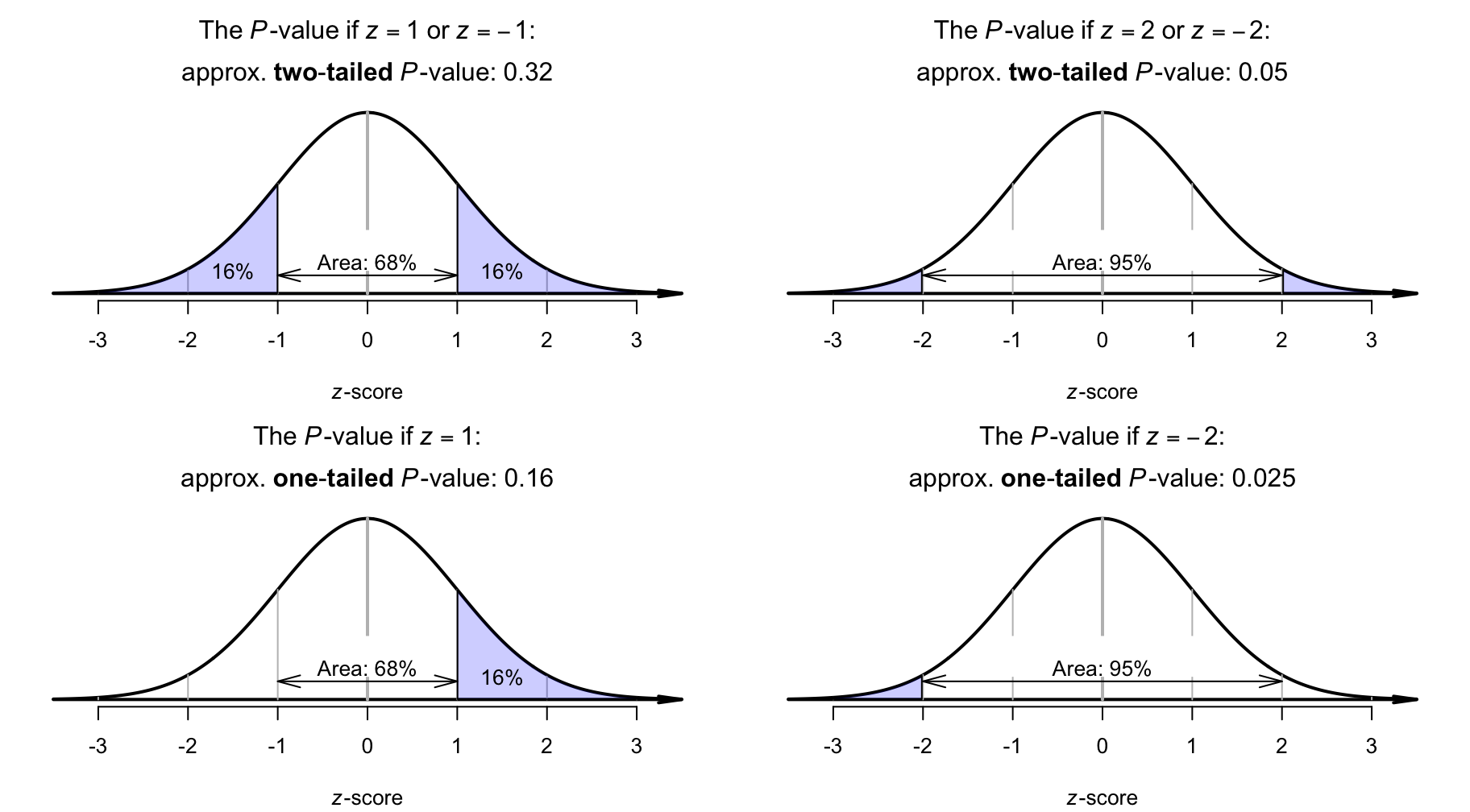
FIGURE 26.3: The two-tailed \(P\)-value is the combined area in the two tails of the distribution. Top left panel: if \(z = 1\) (or \(z = -1\)), the two-tailed \(P\)-value is approximately \(0.16\). Top right panel: if \(z = 2\) (or \(z = -2\)), the two-tailed \(P\)-value is approximately \(0.05\). The corresponding one-tailed \(P\)-values are half the two-tailed \(P\)-values, and are shown in the bottom panels.

Of course, calculated \(z\)-scores are unlikely to be exactly \(z = 1\) or \(z = -2\). Suppose the \(z\)-score is a little larger than \(z = 1\); say \(z = 1.2\). Then, the two-tailed area will be a little smaller than the tail area when \(z = 1\) (Fig. 26.4, left panel). The two-tailed \(P\)-value is a little smaller than \(0.32\).

Similarly, suppose the \(z\)-score is not quite equal to \(z = -2\); say \(z = -1.9\). Then, the two-tailed area will be a little larger than the tail area when \(z = -2\) (Fig. 26.4, right panel). The two-tailed \(P\)-value is a little larger than \(0.05\).

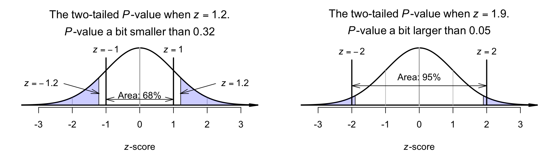
FIGURE 26.4: The two-tailed \(P\)-value for \(z\)-scores not aligned with the \(68\)--\(95\)--\(99.7\) rule. Left panel: when \(z = 1.2\) (or \(z = -1.2\)). Right panel: when \(z = 1.9\) (or \(z = -1.9\)).

26.7.2 More precise \(P\)-values using tables

Using the tables of areas under normal distributions (Appendix B.1.), more precise \(P\)-values can be found using the ideas from Sect. 20.6. For instance (see Fig. 26.4):

• For \(z = 1.2\): the area to the left of \(z = -1.2\) is \(0.1151\), and the area to the right of \(z = 1.2\) is \(0.1151\), so the two-tailed \(P\)-value is \(0.1151 + 0.1151 = 0.2302\). This is a little smaller than \(0.32\), as estimated above.
• For \(z = 1.9\): the area to the left of \(z = -1.9\) is \(0.0287\), and the area to the right of \(z = 1.9\) is \(0.0287\), so the two-tailed \(P\)-value is \(0.0287 + 0.0287 = 0.0574\). This is a little larger than \(0.05\), as estimated above.

In this die-rolling example, where \(z = 4.05\), the tail area is very small (using Appendix B.1), and zero to four decimal places. \(P\)-values are never exactly zero, so we write \(P < 0.0001\) (that is, the \(P\)-value is less than \(0.0001\)).

\(P\)-values tells us the probability of observing the sample statistic (or a value even more extreme), assuming the null hypothesis is true. In the die-rolling example, the \(P\)-value is the probability of observing the value of \(\hat{p} = 0.38\) (or more extreme), just through sampling variation if \(p = 1/6\). Then (see the animation below).

• 'Big' \(P\)-values mean the sample statistic (i.e., \(\hat{p}\)) could reasonably have occurred through sampling variation in one of the many possible samples, if the assumption made about the parameter (stated in \(H_0\)) was true: the data do not contradict the assumption in \(H_0\). There is no persuasive evidence to support the alternative hypothesis.
• 'Small' \(P\)-values mean the sample statistic (i.e., \(\hat{p}\)) is unlikely to have occurred through sampling variation in one of the many possible samples, if the assumption made about the parameter (stated in \(H_0\)) was true: the data do contradict the assumption in \(H_0\). There is persuasive evidence to support the alternative hypothesis.

What is meant by 'small' and 'big' in this context? What represents persuasive evidence to support the alternative hypothesis? A \(P\)-value smaller than \(5\)% (or \(0.05\)) is usually considered 'small', and persuasive evidence to support the alternative hypothesis. In contrast, a \(P\)-value larger than \(5\)% (or \(0.05\)) is usually considered 'big', and not persuasive evidence to support the alternative hypothesis.

The value of \(0.05\) given here is arbitrary, and in some disciplines the distinction is made when \(P = 0.01\) or \(P = 0.10\) instead. Rather than having an arbitrary boundary between 'big' and 'small', a more sensible approach is to qualify the strength of the evidence that supports the alternative hypotheses, which is discussed in Sect. 28.6.

In this die-rolling example, where the \(P\)-value is very small, the data contradict the null hypothesis (that \(p = 1/6\)): the evidence supports the alternative hypothesis that \(p \ne 1/6\). This suggests that the die is very likely not fair.

Be careful interpreting the results! We cannot be sure that the die is unfair. A small \(P\)-value is not proof that the die is loaded. The die may be fair but, due to sampling variation, the sample we observed may simply have produced an unusually high proportion of rolls that show a ⚀ by chance.

The result is interpreted as 'there is evidence that the die is unfair'. Remember: the onus is on the data to refute the null hypothesis, the initial assumption.

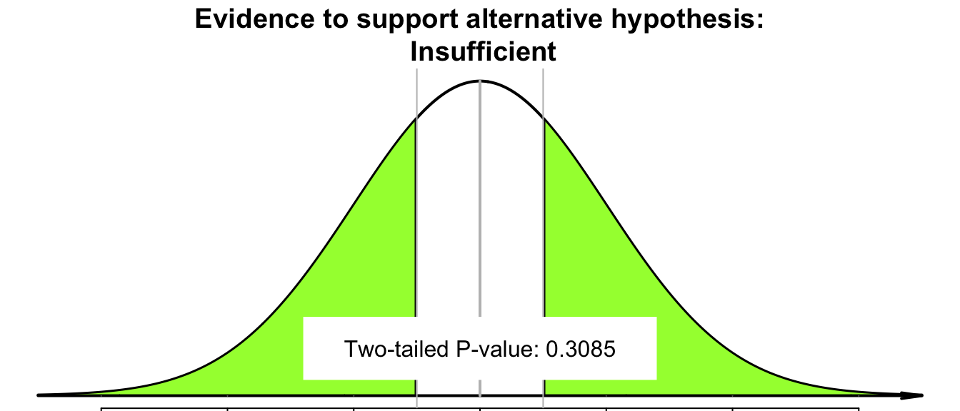
Example 26.1 (Interpreting P-values) In the die example, suppose we found the two-tailed \(P\)-value as \(0.26\). This is relatively 'large' (i.e., much larger than \(0.05\)). Then the observed value of \(\hat{p}\) could easily be explained by chance, and is not persuasive evidence to support the alternative hypothesis (that the die is unfair). There is no evidence that \(p\) is not \(1/6\).

26.8 Writing conclusions

In general, communicating the results of any hypothesis test requires:

• an answer to the RQ, worded in terms of how much evidence exists to support the alternative hypothesis.
• a summary of the evidence used to reach that conclusion (such as the \(z\)-score and \(P\)-value, including if the \(P\)-value is one- or two-tailed).
• sample summary information (see Chap. 22), summarising the data used to make the decision (which usually includes a confidence interval for the parameter).

So for the die-rolling example, write:

The sample provides very strong evidence (\(z = 4.05\); two-tailed \(P < 0.001\)) that the proportion of rolls that show a ⚀ is not \(1/6\) (\(\hat{p} = 0.38\); approx. \(95\)% CI: \(0.243\) to \(0.517\); \(n = 50\) rolls) in the population.

This statement includes the three necessary components:

• an answer to the RQ: 'The sample provides very strong evidence... that the population proportion is not \(1/6\)'.
• the evidence used to reach the conclusion: '\(z = 4.05\); two-tailed \(P < 0.001\)'.
• sample summary information (including a CI).

Since the null hypothesis is initially assumed to be true, the onus is on the evidence to refute the null hypothesis. That is, we retain the null hypothesis unless there is persuasive evidence to stop doing so. Hence, conclusions are worded in terms of how strongly the evidence (i.e., sample data) supports the alternative hypothesis.

The alternative hypothesis may or may not be true, but we report how strongly the evidence (data) supports the alternative hypothesis. Conclusions are not worded in terms of how much evidence support the null hypothesis.

26.9 Process overview

Let's recap the decision-making process, in this context about rolling a ⚀:

1. Assumption: Write the null hypothesis and alternative hypothesis about the parameter (based on the RQ), where \(p\) is the population proportion of rolls that are a ⚀:
   • \(H_0\): \(p = 1/6\) (i.e., sampling variation explains the discrepancy between \(p\) and \(\hat{p}\));
   • \(H_1\): \(p \ne 1/6\) (this is a two-tailed alternative hypothesis).
2. Expectation: The sampling distribution describes what values to reasonably expect from the sample statistic across all possible samples, if the null hypothesis is true. In this situation, the sampling distribution has an approximate normal distribution.
3. Observation: Compute the \(z\)-score (\(z = 4.05\)), a measure of the discrepancy between the assumed population value, and the observed sample value.
4. Decision: Determine if the data are consistent with the assumption, by computing the \(P\)-value. Here, the \(P\)-value is (much) less than \(0.0001\), so very strong evidence exists that \(p\) is not \(1/6\).

26.10 Statistical validity conditions

The hypothesis test conducted in this chapter assumes the sampling distribution is approximately a normal distribution (and so, for example, the \(68\)--\(95\)--\(99.7\) rule can be applied). This is only true if certain conditions are met.

The statistical validity conditions for a test for a single proportion is that the expected number of individuals in the group of interest (i.e, \(n\times p\)) and in the group not of interest (i.e., \(n\times (1 - p)\)) both exceed five; that is:

• Both \(n\times p > 5\), and \(n\times (1 - p) > 5\).

The value of \(5\) here is a rough figure; some books give other values (such as \(10\)). This condition ensures that the sampling distribution of the sample proportions has an approximate normal distribution (so that, for example, the \(68\)--\(95\)--\(99.7\) rule can be used). The units of analysis are also assumed to be independent (e.g., from a simple random sample). For a test for one proportions, these conditions are similar to those for the CI for one proportion (Sect. 22).

If the statistical validity conditions are not met, other similar options include using a binomial test (Conover 2003).

Example 26.2 (Statistical validity) The hypothesis test regarding the dice is statistically valid. Firstly, \(n\times p = 50 \times (1/6) = 8.666\dots\) (i.e., expect about \(8.7\) rolls to show a ⚀), and \(n\times (1 - p) = 41.666\dots\) (i.e., expect about \(41.7\) rolls to not show a ⚀). Both comfortably exceed five, so the normal distribution will be a good approximation for the sampling distribution. This is what we observe from simulation (Fig. 26.5, left panel).

Example 26.3 (Statistical validity) Suppose the die was rolled \(10\) times rather than \(50\) times. Then, \(n\times p = 10 \times (1/6) = 1.666\dots\) and \(n\times (1 - p) = 10 \times (1 - 1/6) = 8.333\dots\). These do not both exceed five, so the normal distribution may be a poor approximation for the sampling distribution.

This is what we observe from simulating the situation (Fig. 26.5, right panel). The normal model is poor: the simulation shows that the sample proportions are not even symmetrically distributed.

(ref:StatValidp) The sampling distributions for two situations for rolling a die. Left: for sets of 50 rolls, the sampling distribution does have an approximate normal distribution. Right: for sets of \(10\) rolls, the sampling distribution does not have a normal distribution. The solid lines show the approximate normal distributions, and the histograms show the distribution of the sample proportions over many sets of rolls. The solid dots are the value \(p = 1/6\), the population proportion of rolls that show a ⚀.

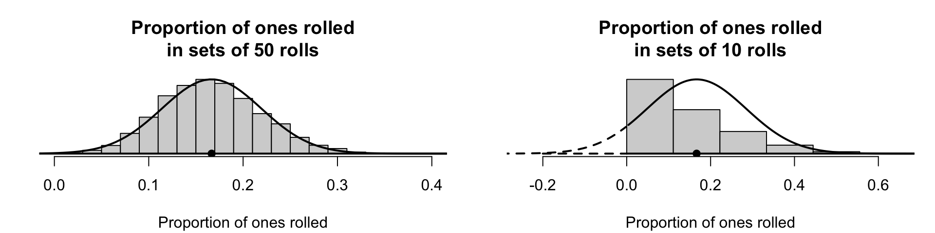
FIGURE 26.5: (ref:StatValidp)

26.11 Example: rolling the other die

In \(50\) rolls of the other die, I found a ⚀ on \(7\) rolls, so that \(\hat{p} = 7/50 = 0.14\). To determine if this die appears loaded, the hypotheses are the same as before: \[ \text{$H_0$: } p = 1/6. \qquad\text{and}\qquad \text{$H_1$: } p \ne 1/6. \] Following the procedures above (check!) and using the same hypotheses, \(z = -0.506\) and (using tables) the two-tailed \(P\)-value is \(2\times 0.3061 = 0.6122\). This means that the sample result was not unusual if \(p = 1/6\), and is certainly not persuasive evidence to support the alternative hypothesis. There is no evidence to suggest the second die is loaded.

This all implies the first die was the loaded die. Now I need to decide how to distinguish the two dice

A large \(P\)-value does not prove that the die is fair! It only means that the proportions of rolls that produce a ⚀ is not unusual... but perhaps the die is loaded in some other way (i.e., to produce more-than-expected rolls of a ⚄).

A large \(P\)-value does not necessarily mean that the die is fair! The die may indeed be loaded to produce a larger-than-expected numbers of rolls that show a ⚀, but (due to sampling variation) the sample we observed simply did not provide evidence to make that conclusion.

The result is interpreted in terms of how much evidence exists to support the alternative hypothesis. The onus is on the data (i.e., evidence) to refute the assumption made in the null hypothesis.

26.12 Example: dominance of birds

Barve and Dhondt (2017) compared two types of birds (male green-backed tits; male cinereous tits) to see which was more behaviourally dominant over winter. If the species were equally-dominant, then about \(50\)% of the interactions would be won by each species. If we define \(p\) as the proportion of interactions won by green-backed tits, then we would expect \(p = 0.50\). However, in the \(45\) interactions observed between the two species, green-backed tits won \(37\) interactions (i.e., \(\hat{p} = 37/45 = 0.82222\)). A discrepancy exists between the sample proportion (\(\hat{p} = 0.8222\)) and the expected population proportion \(p = 0.50\).

Of course, every sample of \(45\) interactions would produce a different value of \(\hat{p}\). To test if the population proportion of interaction wins could be equally shared, the hypotheses are: \[ \text{$H_0$: } p = 0.5\quad\text{and}\quad\text{$H_1$: } p \ne 0.5 \text{ (two-tailed)}. \] The test is statistically valid, since both \(n\times p = 45\times 0.5 = 22.5\) and \(n\times (1 - p) = 22.5\) exceed five. The standard error is \[ \text{s.e.}(\hat{p}) = \sqrt{\frac{p \times (1 - p)}{n}} = \sqrt{\frac{0.50 \times (1 - 0.50)}{45}} = 0.0745356... \] Then, the value of the test statistic is: \[ z = \frac{\hat{p} - p}{\text{s.e.}(\hat{p})} = \frac{0.82222 - 0.50}{0.0745356} = 4.322. \] This is a very large \(z\)-score, so the \(P\)-value will be very small, using the \(68\)--\(95\)--\(99.7\) rule, or using tables. This is persuasive evidence to support the alternative hypothesis. We write:

Very strong evidence exists in the sample (\(P < 0.0001\); \(z = 4.325\)) that the interactions were not won equally by each species (\(\hat{p} = 0.8222\) won by green-backed tits; approx. \(95\)% CI: \(0.708\) to \(0.936\); \(n = 45\)) in the population.

26.13 Chapter summary

To test a hypothesis about a population proportion \(p\):

• Write the null hypothesis (\(H_0\); the sampling variation explanation) and the alternative hypothesis (\(H_1\)).
• Initially assume the value of \(p\) in the null hypothesis to be true.
• Then, describe the sampling distribution, which describes what to expect from the sample statistic across all possible samples, based on this assumption: under certain statistical validity conditions, the sample mean varies with:
  • an approximate normal distribution,
  • with sampling mean, whose value is the value of \(p\),
  • with a standard deviation of \(\displaystyle \text{s.e.}(\hat{p}) = \sqrt{\frac{p \times (1 - p)}{n}}\), where \(p\) is the hypothesised value given in the null hypothesis, and \(n\) is the sample size.
• Compute the value of the test statistic: \[ z = \frac{ \hat{p} - p}{\text{s.e.}(\hat{p})}. \]
• Compute an approximate \(P\)-value using the \(68\)--\(95\)--\(99.7\) rule, or using tables.
• Make a decision, and write a conclusion.
• Check the statistical validity conditions.

26.14 Quick review questions

A study of diseases in Native Americans (Kizer et al. 2006) found \(381\) obese or overweight patients in \(449\) patients. In the general population of the USA, the percentage obese or overweight was \(65\)%. The researchers wanted to determine if the percentage of obesity/overweight Native Americans was greater than that of the general population.

Are the following statements true or false?

1. The sample size is \(n = 381\). TRUE FALSE
2. The value of the sample proportion is \(\hat{p} = 381\). TRUE FALSE
3. The null hypothesis is \(H_0\): \(p = 0.65\). TRUE FALSE
4. The alternative hypothesis is \(H_0\): \(p = 0.8486\). TRUE FALSE
5. We initially assume the population proportion of overweight/obese Native Americans is \(0.65\). TRUE FALSE
6. The alternative hypothesis is one-tailed. TRUE FALSE
7. In a one-sample test of proportion, the \(z\)-score is always large. TRUE FALSE
8. The value of the \(z\)-score for this example is \(8.82\). TRUE FALSE
9. We have evidence to support the alternative hypothesis in this example. TRUE FALSE
10. We always accept the null hypothesis. TRUE FALSE

26.15 Exercises

Answers to odd-numbered exercises are given at the end of the book.

Exercise 26.1 Explain why the standard error is computed using \(p\) for hypothesis testing, but using \(\hat{p}\) for confidence intervals.

Exercise 26.2 Explain why describing the sampling distribution is difficult if we assume \(p \ne 1/6\).

Exercise 26.3 In the die example, the observed proportion is \(0.38\). Explain why we cannot simply state that the proportion clearly is not \(1/6 = 0.1666\) (as it is clearly \(0.38\)).

Exercise 26.4 Explain why we compute \(\text{s.e.}(\hat{p})\) and not \(\text{s.e.}(p)\).

Exercise 26.5 What is wrong with the following statement, after testing \(H_0\): \(p = 0.25\):

There is very strong evidence that the sample proportion is greater than \(0.25\).

Exercise 26.6 Explain what is wrong with this statement from Davis et al. (2024), that appears under their Table 2:

One proportion \(z\)-test with \(H_0 = 0.076\), the proportion of UDT in our sample

Exercise 26.7 The study of herbal medicines is complicated, as blinding subjects is difficult: placebos are often easily identifiable by eye, by taste, or by smell.

Loyeung et al. (2018) studied if subjects could identify potential placebos at a better rate than just guessing. The \(81\) subjects were each presented with a choice of five different supplements, four of which were placebos. Subjects were asked to select which one was the legitimate herbal supplement based on the taste. Of these, \(50\) correctly selected the true herbal supplement.

1. If the subjects were selecting the true herbal supplement randomly, what proportion of subjects would be expected to select the correct supplement as the true herbal medicine?
2. Write the hypotheses for addressing the aims of the study.
3. Is this a one- or two-tailed test? Explain.
4. Sketch the sampling distribution of the sample proportion, assuming \(H_0\) is correct.
5. Is there evidence that people can identify the true supplement by taste?
6. Are the statistical validity conditions satisfied?

Exercise 26.8 S.-S. Kim et al. (2004) studied the measles-rubella vaccination-rates in Korea, comparing the proportion of children susceptible to measles with the World Health Organization target proportion (for children aged \(5\) to \(9\) years old: \(10\)%).

The aim was to test if the proportion of Korean children susceptible to measles in the population was \(10\)% or lower (i.e., better). In the study, \(55\) children out of \(972\) were susceptible to measles.

1. Compute the sample proportion \(\hat{p}\) of children susceptible to measles.
2. Write the hypotheses for the test. Is the test one- or two-tailed?
3. Compute the standard error for the test.
4. Compute the \(z\)-score and determine the \(P\)-value.
5. Write a conclusion.
6. Are the statistical validity conditions satisfied?

Exercise 26.9 Streeting et al. (2022) studied western saw-shelled turtles. When eggs were incubated at \(27\)^oC, they observed that \(29\) males and \(44\) females hatched. Are the proportions of male and female turtles that hatch at this temperature equal?

Exercise 26.10 [Dataset: PremierL] In the 2019/2020 English Premier League (EPL), the home team won \(91\) games, and the away team won \(67\) games. (Another \(50\) games were draws.)

Use the \(n = 158\) games with a result to determine if there is evidence that the home team wins more often than \(50\)% (i.e., that there is a home-side advantage).

Exercise 26.11 Maeda (2013) introduced pedal machines on the first floor of the Joyner Library for use by students at East Carolina University (ECU) to increase activity in library users. At ECU, \(60.2\)% of all students were females (i.e., in the population). Students were observed using the machine on \(589\) occasions, of which \(295\) times were by females

Is there evidence that the proportion of female users of the machines was lower than the overall female proportion at the university? What would you conclude?

Exercise 26.12 Koenen (1995) found that \(88\) of the \(357\) visitors to Las Vegas casinos in 1995 were smokers. At the time, \(25.5\)% of the general US population were smokers (based on data from the US National Center for Health Statistics). Is the proportion of smokers among casino-goers the same as for the general US population?

Exercise 26.13 Nochera and Ragone (2019) developed gluten-free pasta made from breadfruit. In the study sample, \(57\) of the \(71\) participants stated that they liked the pasta. Do the researchers have sufficient evidence to claim that the 'majority of people like breadfruit pasta'?

Exercise 26.14 Carpal Tunnel Syndrome (CTS) is a painful condition in the wrists. Boltuch et al. (2020) were interested in whether 'a relationship exists between the palmaris tendon [and] carpal tunnel syndrome (CTS)' (p. 493). The palmaris longus (PL) tendon is visually absent in about \(15\)% of the population. The researchers found PL was visually absent in \(33\) of \(516\) CTS wrists in their sample. Is there evidence to suggest that rate of PL absence is different in CTS cases, compared to the general population?

Exercise 26.15 Siegfried et al. (2014) studied resistance of some commercial corn varieties to the European corn borer. Borers were collected from corn in Iowa and Nebraska.

Researchers aimed to estimate the frequency of resistance to the toxin in the corn. By mating borers collected from the field with various resistant laboratory individuals, they could determine what proportion of resistant individuals to expect in the second generation offspring. In one study of \(n = 172\) second-generation individuals, \(24\) were found to be resistant. The expectation was that \(1\)-in-\(16\) of the second-generation borers would be resistant if the field borers were resistant. Perform a hypothesis test to determine if the data suggest that the field borers were resistant (that is, if the population proportion is \(1/16\)) as expected.

Exercise 26.16 Davidovic et al. (2019) studied street-light preferences of drivers. Drivers were asked to conduct a series of manoeuvres under \(3\,000\)K LED light and then under \(4\,000\)K LED lights. They were then asked to decide which street light they preferred. Out of the \(52\) subjects, \(29\) preferred the \(3\,000\)K LED lights. Is there evidence that the choice between the two street lights is random, or is there evidence of a preference for one over the other?

Exercise 26.17 The euro was introduced as a currency on 01 January 1999. According to a report by the New Scientist, students in Poland spun a Belgian one-euro coin \(250\) times, and found \(140\) heads (as reported by Gelman and Nolan (2002)). This resulted in an 'accusation of bias' in the New Scientist article. However, every set of \(250\) spins can produce a different proportion of heads, so perhaps the results is just due to randomness. Does this sample of \(250\) spins suggest that the one-euro Belgian coin is biased?

Exercise 26.18 As noted in Sect. 18.3.2, the Australian Bureau of Statistics (ABS) stated that:

The sex ratio for all births registered in Australia generally fluctuates around \(105.5\) male births per \(100\) female births.

(This statistic does not use births registered as 'other' or 'not stated'.)

1. The value of \(105.5\) is effectively a population odds ratio of male-to-female births. Show that this is equivalent to the population proportion of male births as \(0.51338\) (not including 'other' or 'not stated').
2. In 2021, there were \(148\,636\) male births and \(140\,944\) female births. Compute the sample proportion of male births in 2021 (to five decimal places).
3. Conduct a test to determine if the 2021 data appear different to the long-term proportion.

---

Peter K. Dunn, 2024: CC BY-NC-SA 4.0