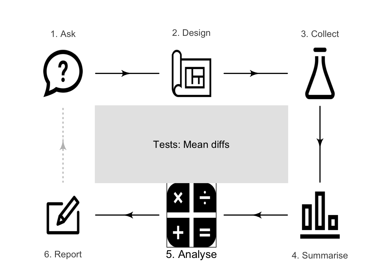
33 Tests for the mean difference (paired data)

You have learnt to ask a RQ, design a study, classify and summarise the data, construct confidence intervals, and perform some hypothesis tests. In this chapter, you will learn to:

• identify situations where conducting a test for a proportion is appropriate.
• conduct hypothesis tests for the mean difference with paired data
• determine whether the conditions for using these methods apply in a given situation.

33.1 Introduction: soil nitrogen

Lambie, Mudge, and Stevenson (2021) compared the percentage nitrogen (%N) in soils from irrigated and non-irrigated intensively-grazed pastures. The researchers paired similar irrigated and non-irrigated sites (p. 338):

The irrigated and non-irrigated pairs within each site were within \(100\) m of each other and were on the same soil, landform and usually the same farm with the same farm management on both treatments.

Pairing (Sect. 26.1) is a form of blocking (Sect. 7.2) and is used to manage confounding. One RQ in the study was:

For intensively grazed pastures sites, is there a mean reduction in percentage soil nitrogen (%N) when sites are irrigated, compared to non-irrigated?

The data are shown in the table below. The parameter is \(\mu_d\), the population mean reduction in %N when sites are irrigated, compared to non-irrigated.

Explaining how the differences are computed is important.
The differences here are the %N in non-irrigated sites minus %N in irrigated sites.

The differences could be computed as the %N in irrigated sites minus %N in non-irrigated sites. Either is fine, as long as you remain consistent throughout. The meaning of any conclusions will be the same.

TABLE 33.1: The percentage total nitrogen in irrigated and non-irrigated soils in \(n = 28\) sites

Irrigated	Not irrigated	Reduction
\(\phantom{0}0.35\)	\(\phantom{0}0.38\)	\(\phantom{-}0.03\)
\(\phantom{0}0.42\)	\(\phantom{0}0.43\)	\(\phantom{-}0.01\)
\(\phantom{0}0.27\)	\(\phantom{0}0.23\)	\(-0.04\)
\(\phantom{0}0.18\)	\(\phantom{0}0.24\)	\(\phantom{-}0.06\)
\(\phantom{0}0.56\)	\(\phantom{0}0.58\)	\(\phantom{-}0.02\)
\(\phantom{0}0.34\)	\(\phantom{0}0.26\)	\(-0.08\)
\(\phantom{0}0.26\)	\(\phantom{0}0.25\)	\(-0.01\)
\(\phantom{0}0.58\)	\(\phantom{0}0.44\)	\(-0.14\)
\(\phantom{0}0.50\)	\(\phantom{0}0.49\)	\(-0.01\)
\(\phantom{0}0.47\)	\(\phantom{0}0.55\)	\(\phantom{-}0.08\)
\(\phantom{0}0.55\)	\(\phantom{0}0.55\)	\(\phantom{-}0.00\)
\(\phantom{0}0.41\)	\(\phantom{0}0.45\)	\(\phantom{-}0.04\)
\(\phantom{0}0.51\)	\(\phantom{0}0.54\)	\(\phantom{-}0.03\)
\(\phantom{0}0.47\)	\(\phantom{0}0.56\)	\(\phantom{-}0.09\)
\(\phantom{0}0.27\)	\(\phantom{0}0.33\)	\(\phantom{-}0.06\)
\(\phantom{0}0.29\)	\(\phantom{0}0.31\)	\(\phantom{-}0.02\)
\(\phantom{0}0.40\)	\(\phantom{0}0.43\)	\(\phantom{-}0.03\)
\(\phantom{0}0.26\)	\(\phantom{0}0.26\)	\(\phantom{-}0.00\)
\(\phantom{0}0.52\)	\(\phantom{0}0.53\)	\(\phantom{-}0.01\)
\(\phantom{0}0.30\)	\(\phantom{0}0.41\)	\(\phantom{-}0.11\)
\(\phantom{0}0.20\)	\(\phantom{0}0.32\)	\(\phantom{-}0.12\)
\(\phantom{0}0.30\)	\(\phantom{0}0.30\)	\(\phantom{-}0.00\)
\(\phantom{0}0.24\)	\(\phantom{0}0.26\)	\(\phantom{-}0.02\)
\(\phantom{0}0.49\)	\(\phantom{0}0.67\)	\(\phantom{-}0.18\)
\(\phantom{0}0.27\)	\(\phantom{0}0.29\)	\(\phantom{-}0.02\)
\(\phantom{0}0.44\)	\(\phantom{0}0.47\)	\(\phantom{-}0.03\)
\(\phantom{0}0.27\)	\(\phantom{0}0.28\)	\(\phantom{-}0.01\)
\(\phantom{0}0.40\)	\(\phantom{0}0.50\)	\(\phantom{-}0.10\)

The data are summarised graphically (Fig. 33.1) and numerically (Table 33.2), using information provided by software (Fig. 33.2).

TABLE 33.2: The percentage total soil N in irrigated and non-irrigated sites

	Mean	Std. dev.	Std. error	Sample size
Irrigated sites	\(0.3757\)	\(0.1186\)	\(0.0224\)	\(28\)
Non-irrigated sites	\(0.4039\)	\(0.1266\)	\(0.0239\)	\(28\)
Change	\(0.0282\)	\(0.0618\)	\(0.0117\)	\(28\)

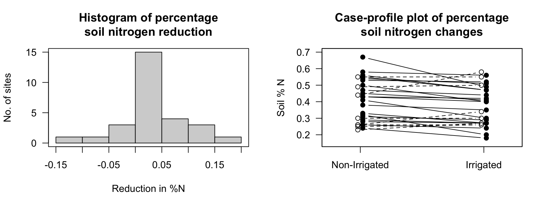
FIGURE 33.1: The reduction in %N when sites are irrigated, compared to non-irrigated. Left: A histogram of the differences (boundary values in the lower box). Right: a case-profile plot (solid lines, solid dots for lower percentage N in irrigated sites).

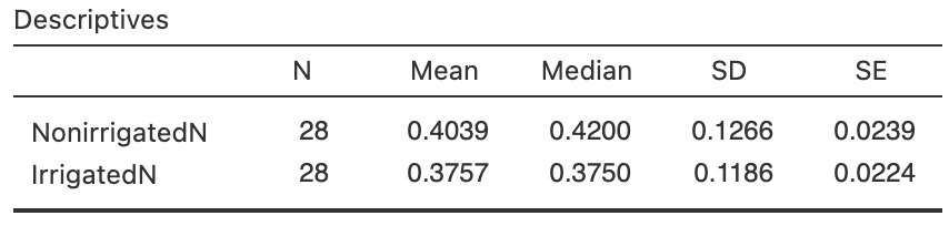
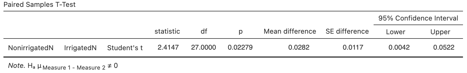
FIGURE 33.2: jamovi output for the nitrogen data

33.2 Statistical hypotheses and notation

The RQ asks if the mean %N reduces in the population when sites are irrigated. If the differences are defined as the %N for non-irrigated sites minus irrigated sites, then positive values refer to non-irrigated sites having larger %N than irrigated sites, on average. Then, the RQ is asking if the mean difference is zero, or if it is greater than zero. The parameter is the population mean difference. The notation used (recapping Sect. 26.4) is:

• \(\mu_d\): the mean difference in the population (in %N).
• \(\bar{d}\): the mean difference in the sample (in %N).
• \(s_d\): the sample standard deviation of the differences (in %N).
• \(n\): the number of differences.

The null hypothesis is that 'there is no mean change in %N, in the population' (Sect. 32.2):

• \(H_0\): \(\mu_d = 0\).

This hypothesis, which we initially assume to be true, postulates that the mean reduction may not be zero in the sample, due to sampling variation.

Since the RQ asks specifically if mean %N decreases, the alternative hypothesis is one-tailed (Sect. 32.2). According to how the differences have been defined, the alternative hypothesis is:

• \(H_1\): \(\mu_d > 0\) (i.e., one-tailed).

This hypothesis says that the mean change in the population is greater than zero, because of the wording of the RQ, and because of how the differences were defined. (If the differences were defined in the opposite way---as '%N in irrigated sites minus non-irrigated sites'--- then the alternative hypothesis would be \(\mu_d < 0\), which has the same meaning.)

33.3 Tests for the mean difference: \(t\)-test

The sample mean %N reduction varies depending on which one of the countless possible samples is randomly obtained, even if the mean reduction in the population is zero. That is, the value of \(\bar{d}\) varies across all possible samples even if \(\mu_d = 0\). The value of \(\bar{d}\) has a sampling distribution.

Definition 33.1 (Sampling distribution of a sample mean difference) The sampling distribution of the sample mean difference is (when certain conditions are met; Sect. 33.5) described by

• an approximate normal distribution,
• centred around the sampling mean difference, whose value is \(\mu_d\) (from \(H_0\)),
• with a standard deviation (called the standard error of \(\bar{d}\)) of
  \[\begin{equation} \text{s.e.}(\bar{d}) = \frac{s_d}{\sqrt{n}}, \tag{33.1} \end{equation}\] where \(n\) is the number of differences, and \(s_d\) is the standard deviation of the differences.

The value of the standard error of the differences here is \[ \text{s.e.}(\bar{d}) = s_d/\sqrt{n} = 0.0618/\sqrt{28} = 0.0117. \] This sampling distribution of \(\bar{d}\) is shown in Fig. 33.3.

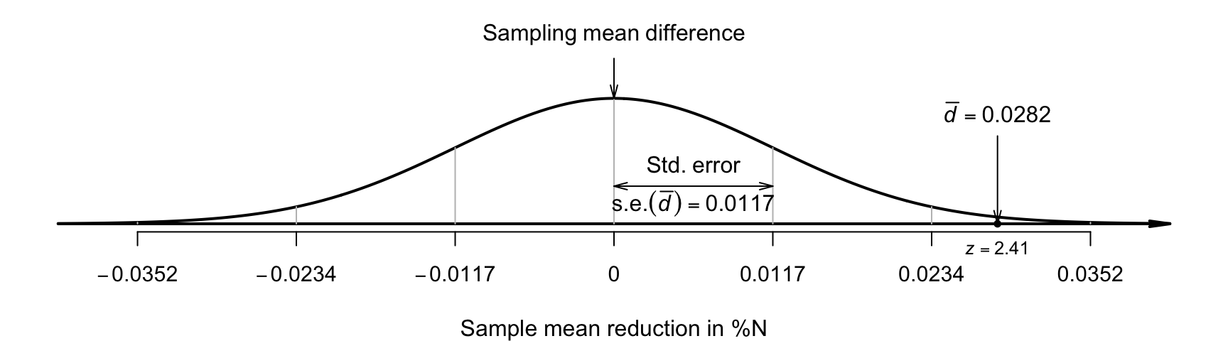
FIGURE 33.3: The sampling distribution is a normal distribution; it describes how the sample mean reduction in percentage N varies in samples of size \(n = 28\) when the population mean reduction is \(0\).

The sample mean difference can be located on the sampling distribution (Fig. 33.3) by computing the \(t\)-score: \[ t = \frac{\bar{d} - \mu_{d}}{\text{s.e.}(\bar{d})} = \frac{0.0282 - 0}{0.0117} = 2.41, \] following the ideas in Eq. (31.2). Software also displays the \(t\)-score (Fig. 33.2).

A \(P\)-value determines if the sample data are consistent with the assumption (Table 32.1). Since \(t = 2.41\), and since \(t\)-scores are like \(z\)-scores, the one-tailed \(P\)-value is smaller \(0.025\) (based on the \(68\)--\(95\)--\(99.7\) rule). Software (Fig. 33.2) reports that the two-tailed \(P\)-value is \(0.02279\). Hence, the one-tailed \(P\)-value is \(0.02279/2 = 0.0114\).

The jamovi software clarifies how the differences have been computed. At the left of the output (Fig. 33.2), the order implies the differences are found as NonirrigatedN minus IrrigatedN, the same as our definition.

33.4 Writing conclusions

The one-tailed \(P\)-value is \(0.0114\), suggesting moderate evidence (Table 32.1) to support \(H_1\). A conclusion requires an answer to the RQ, a summary of the evidence leading to that conclusion, and some summary statistics:

Moderate evidence exists in the sample (paired \(t = 2.41\); one-tailed \(P = 0.0114\)) of a mean reduction in percentage soil N from non-irrigated to irrigated sites (mean reduction: \(0.0282\)%; \(n = 28\); \(95\)% CI from \(0.0042\)% to \(0.0522\)%).

The CI is found using the process described in Chap. 26.1. The wording implies the direction of the differences.

Saying 'there is evidence of a difference' is insufficient. You must state which measurement is, on average, higher (that is, what the differences mean).

33.5 Statistical validity conditions

As with any hypothesis test, these results apply under certain conditions. For a hypothesis test for the mean of paired data, these conditions are the same as for the CI for the mean difference for paired data (Sect. 26.5), and similar to those for one sample mean.

Statistical validity can be assessed using these criteria:

• When \(n > 25\), the test is statistically valid provided the distribution of differences is not highly skewed.
• When \(n \le 25\), the test is statistically valid only if the data come from a population of differences with a normal distribution.

The sample size of \(25\) is a rough figure; some books give other values (such as \(30\)). Data with severe skewness or large outliers may need a larger sample size for the test to be statistically valid.

This condition ensures that the distribution of the sample mean differences has an approximate normal distribution (so that, for example, the \(68\)--\(95\)--\(99.7\) rule can be used). Provided \(n > 25\), this will be approximately true even if the distribution of the differences in the population does not have a normal distribution.

If the statistical validity conditions are not met, other similar options include using a sign test of the differences or a Wilcoxon signed-rank test of the differences (Conover 2003), or using resampling methods (Efron and Hastie 2021).

Example 33.1 (Statistical validity) For the %N data, the sample size is \(n = 28\), so the test is statistically valid.

33.6 Example: invasive plants

(This study was seen in Sect. 26.6.) Skypilot is a alpine wildflower native to the Colorado Rocky Mountains (USA). In recent years, a willow shrub (Salix) has been encroaching on skypilot territory and, because willow often flowers early, Kettenbach et al. (2017) studied whether the willow may 'negatively affect pollination regimes of resident alpine wildflower species' (p. 6965).

Data for both species was collected at \(n = 25\) different sites, so the data are paired by site (Sect. 26.1). The data are shown in Sect. 26.6. The parameter is \(\mu_d\), the population mean difference in day of first flowering for skypilot, less the day of first flowering for willow. A positive value for the difference means that the skypilot values are larger, and hence that willow flowered first. The RQ is:

In the Colorado Rocky Mountains, is there a mean difference between first-flowering day for the native skypilot and encroaching willow?

The hypotheses are \[ \text{$H_0$: $\mu_d = 0$}\quad\text{and}\quad\text{$H_1$: $\mu_d\ne 0$} \] where the alternative hypothesis is two-tailed.

Explaining how the differences are computed is important. The differences here are skypilot minus willow first-flowering days.

However, the differences could be computed as willow minus skypilot first-flowering days. Either is fine, as long as you remain consistent. The meaning of any conclusions will be the same.

The data are summarised graphically in Fig. 14.4. The numerical summary (Table 33.3) and software output (Fig. 33.4) are repeated here.

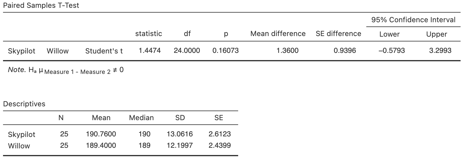
FIGURE 33.4: jamovi output for the flowering-day data

TABLE 33.3: The day of first flowering for encroaching willow and native skypilot

	Mean	Std. dev.	Std. error	Sample size
Willow (encroaching)	\(189.40\)	\(12.200\)	\(2.440\)	\(25\)
Skypilot (native)	\(190.76\)	\(13.062\)	\(2.612\)	\(25\)
Differences	\(\phantom{0}\phantom{0}1.36\)	\(\phantom{0}4.698\)	\(0.940\)	\(25\)

The standard error of the mean difference is \(\text{s.e.}(\bar{d}) = 0.9396\) (Fig. 14.3 or Table 14.4). The value of the test statistic (i.e., the \(t\)-score) is \[\begin{align*} t = \frac{\bar{d} - \mu_d}{\text{s.e.}(\bar{d})} = \frac{1.36 - 0}{0.9396} = 1.45, \end{align*}\] as in the output. This is a relatively small value of \(t\), so a large \(P\)-value is expected using the \(68\)--\(95\)--\(99.7\) rule. Indeed, the output shows that \(P = 0.161\): there is no evidence of a mean difference in first-flowering day (i.e., the sample mean difference could reasonably be explained by sampling variation if \(\mu_d = 0\)). We write:

No evidence exists (\(t = 1.45\); two-tailed \(P = 0.161\)) that the day of first-flowering is different for the encroaching willow and the native skypilot (mean difference: \(1.36\) days earlier for willow; \(95\)% CI from \(-0.57\) to \(3.30\); \(n = 25\)).

The test is statistically valid since \(n = 25\).

We do not say whether the evidence supports the null hypothesis. We assume the null hypothesis is true, so we state how strong the evidence is to support the alternative hypothesis. The current sample presents no evidence to contradict the assumption, but future evidence may emerge. That is:

No evidence of a difference does not mean evidence of no difference.

Be clear in your conclusion about how the differences are computed. Make sure to interpret the CI consistent with how the differences were defined.

33.7 Example: chamomile tea

(This study was seen in Sects. 26.7 and 27.8.) Rafraf, Zemestani, and Asghari-Jafarabadi (2015) studied patients with Type 2 diabetes mellitus (T2DM). They randomly allocated \(32\) patients into a control group (who drank hot water), and another \(32\) patients to receive chamomile tea. Summary data are shown in Table 26.3.

In Sect. 26.7, a CI was formed for the mean reduction in total glucose (TG) for the hot water and the tea groups separately. However, we can also ask about whether the mean differences in TG are non-zero due to sampling variation or not. The following descriptive RQs can be asked:

• For patients with T2DM, is there a mean change in TG after eight weeks drinking chamomile tea?
• For patients with T2DM, is there a mean change in TG after eight weeks drinking hot water?

The hypotheses are:

\[\begin{align*} \text{Chamomile tea group}: \qquad & \text{$H_0$: } \mu_d = 0\quad \text{vs}\quad\text{$H_1$: } \mu_d \ne 0;\\ \text{Hot water group:}. \qquad & \text{$H_0$: } \mu_d = 0\quad \text{vs}\quad\text{$H_1$: } \mu_d \ne 0. \end{align*}\]

For the two groups, the test statistics are (using the standard errors in Sect. 26.7): \[ t_T = \frac{38.62 - 0}{5.37} = 7.19\qquad\text{and}\qquad t_W = \frac{-7.12 - 0}{6.48} = -1.10, \] where the subscripts \(T\) and \(W\) refer to the tea and hot-water groups respectively. The \(t\)-score for the tea-drinking group is huge, so the two-tailed \(P\)-value will be very small using the \(68\)--\(95\)--\(99.7\) rule, and certainly smaller than \(0.001\). This means that there is evidence that chamomile tea had an impact on the mean change in TG.

In contrast, the \(t\)-score for the water-drinking group is small, so the two-tailed \(P\)-value will be large using the \(68\)--\(95\)--\(99.7\) rule, and certainly larger than \(0.10\). This means there is no evidence that placebo treatment (hot water) had any impact on mean change in TG (as one might expect for a placebo).

We can write:

There is very strong evidence (\(t = 7.19\); two-tailed \(P < 0.001\)) of a mean change in TG for the chamomile-drinking groups (mean reduction: \(38.62\) mg.dl^\(-1\); \(n = 32\); approx. \(95\)% CI: \(27.88\) to \(49.36\) mg.dl^\(-1\)), but no evidence (\(t = -1.10\); two-tailed \(P > 0.10\)) of a mean change in the hot-water drinking group (mean reduction: \(-7.12\) mg.dl^\(-1\); \(n = 32\); approx. \(95\)% CI: \(-20.08\) to \(5.84\) mg.dl^\(-1\)).

The sample sizes are larger than \(25\), so the results are statistically valid.

The two groups appear to show different mean reductions in TG, depending on which group the subject is in. This may suggest that chamomile tea reduces TG compared to the control... but perhaps the difference in TG between the hot water and tea groups is simply due to sampling variation. This is considered in Sect. 34.6.

33.8 Chapter summary

To test a hypothesis about a population mean difference \(\mu_d\):

• Write the null hypothesis (\(H_0\)) and the alternative hypothesis (\(H_1\)).
• Initially assume the value of \(\mu_d\) in the null hypothesis to be true.
• Then, describe the sampling distribution, which describes what to expect from the sample mean difference based on this assumption: under certain statistical validity conditions, the sample mean difference varies with:
  • an approximate normal distribution,
  • with sampling mean whose value is the value of \(\mu_d\) (from \(H_0\)), and
  • having a standard deviation of \(\displaystyle \text{s.e.}(\bar{d}) =\frac{s_d}{\sqrt{n}}\).
• Compute the value of the test statistic: \[ t = \frac{ \bar{d} - \mu}{\text{s.e.}(\bar{d})}, \] where \(\mu_d\) is the hypothesised value given in the null hypothesis.
• The \(t\)-value is like a \(z\)-score, and so an approximate \(P\)-value can be estimated using the \(68\)--\(95\)--\(99.7\) rule, or found using software.

The following short video may help explain some of these concepts:

33.9 Quick review questions

Bacho et al. (2019) compared joint pain in stroke patients before and after a supervised exercise treatment. The same participants (\(n = 34\)) were assessed before and after treatment.

The mean improvement in joint pain after \(13\) weeks was \(1.27\) (with a standard error of \(0.57\)) measured using a standardised tool.

1. True or false: Only 'before and after' studies can be paired. TRUE FALSE
2. True or false: The null hypothesis is about the population mean difference. TRUE FALSE
3. What is the value of the test statistic (to two decimal places)?
4. What is the value of the two-tailed \(P\)-value? Very small Small About 0.05 Large Very large
5. True or false: The 'test statistic' is a \(t\)-score for this test. TRUE FALSE

33.10 Exercises

Answers to odd-numbered exercises are available in App. E.

Exercise 33.1 A group of primary school children were asked to complete a certain task on both a personal computer (PC) and using a tablet computer.

If the differences were defined as the time to complete the task on the PC, minus the time to complete the same task on a tablet (one difference for each child), what do the difference mean?

Exercise 33.2 Suppose water quality was recorded \(500\) m upstream and \(500\) m downstream of \(28\) different copper mines.

If the differences were defined as the pH downstream minus the water pH upstream for each river, what do the differences mean?

Exercise 33.3 [Dataset: Fruit] (These data were also seen in Exercise 26.3.) Mukherjee, Deb, and Devy (2019) studied the effect of rainfall on growing Chayote squash (Sechium edule). They compared the size of the fruit in a year with normal rainfall (2015) compared to a dry year (2014) on \(24\) farms:

For Chayote squash grown in Bangalore, what is the mean difference in fruit weight between a normal and dry year?

Ten fruits were gathered from each farm in both years, and the average (mean) weight of the fruit recorded for the farm. Since the same farms are used in both years, the data are paired (Exercise 26.3). Data is missing for Farm 20 in the dry year (2014), so there are \(n = 23\) differences.

1. Construct a suitable graph for the differences.
2. What is the parameter? Carefully describe what it means.
3. Write down the hypotheses.
4. Compute the \(t\)-score.
5. Determine the \(P\)-value.
6. Write a conclusion.
7. Is the test statistically valid?

Exercise 33.4 (This study was also seen in Exercise 26.4.) In a study of hypertension (Hand et al. 1996; MacGregor et al. 1979), patients were given a drug (Captopril) and their systolic blood pressure measured (in mm Hg) immediately before and two hours after being given the drug (data with Exercise 26.4).

The aim is to see if there is evidence of a reduction in blood pressure after taking Captopril. Using these data (Table 14.6) and the software output (Fig. 33.5):

1. Explain why it is probably more sensible to compute differences as the Before minus the After measurements. What do the differences mean when computed this way?
2. What is the parameter? Carefully describe what it means.
3. Construct a suitable graph for the differences.
4. Write down the hypotheses.
5. Write down the \(t\)-score.
6. Write down the \(P\)-value.
7. Write a conclusion.
8. Is the test statistically valid?

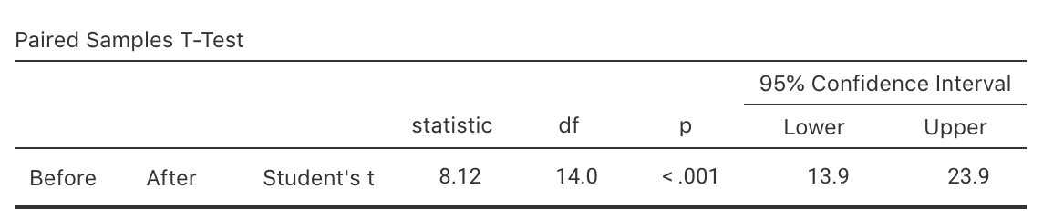
FIGURE 33.5: jamovi output for the Captopril data

Exercise 33.5 (These data were also seen in Exercise 26.5.) People often struggle to eat the recommended intake of vegetables. Fritts et al. (2018) explored ways to increase vegetable intake in teens. Teens rated the taste of raw broccoli, and raw broccoli served with a specially-made dip.

Each teen (\(n = 100\)) had a pair of measurements: the taste rating of the broccoli with and without dip. Taste was assessed using a '\(100\) mm visual analog scale', where a higher score means a better taste. In summary:

• For raw broccoli, the mean taste rating was \(56.0\) (with a standard deviation of \(26.6\));
• For raw broccoli served with dip, the mean taste rating was \(61.2\) (with a standard deviation of \(28.7\)).

Because the data are paired, the differences are the best way to describe the data. The mean difference in the ratings was \(5.2\), with standard error of \(3.06\).

Perform a hypothesis test to see if the use of dip increases the mean taste rating.

Exercise 33.6 (This study was also seen in Exercise 26.6.) Allen et al. (2018) examined the effect of exercise on smoking. Men and women were assessed on their 'intention to smoke', both before and after exercise for each subject (using two quantitative questionnaires). Smokers ('smoking at least five cigarettes per day') aged \(18\) to \(40\) were enrolled for the study. For the \(23\) women in the study, the mean intention to smoke after exercise reduced by \(0.66\) (with a standard error of \(0.37\)).

Perform a hypothesis test to determine if there is evidence of a population mean reduction in intention-to-smoke for women after exercising.

Exercise 33.7 In a study (Cressie, Sheffield, and Whitford 1984) conducted at the Adelaide Children's Hospital (p. 107; emphasis added):

...a group of beta thalassemia patients [...] were treated by a continuous infusion of desferrioxamine, in order to reduce their ferritin content...

Using the data shown below, conduct a hypothesis test to determine if there is evidence that the treatment reduces the ferritin content, as intended.

TABLE 33.4: The ferritin content (in \(\mu\)g/L) for 20 thalassemia patients at the Adelaide Children's Hospital (first ten observations)

September	March	Reduction
\(6630\)	\(5100\)	\(\phantom{-}1530\)
\(4590\)	\(3510\)	\(\phantom{-}1080\)
\(3510\)	\(6600\)	\(-3090\)
\(6375\)	\(8000\)	\(-1625\)
\(2500\)	\(2800\)	\(-300\)
\(1400\)	\(2860\)	\(-1460\)
\(4580\)	\(3640\)	\(\phantom{-}\phantom{0}940\)
\(6885\)	\(9030\)	\(-2145\)
\(4200\)	\(4420\)	\(-220\)
\(5600\)	\(7910\)	\(-2310\)

Exercise 33.8 (This study was also seen in Exercise 26.8.) The concentration of beta-endorphins in the blood is a sign of stress. Hoaglin, Mosteller, and Tukey (2011) measured the beta-endorphin concentration for \(19\) patients about to undergo surgery (Hand et al. 1996). Each patient had their beta-endorphin concentrations measured \(12\)--\(14\) hours before surgery, and also \(10\) minutes before surgery.

A numerical summary (Table 33.5) can be produced from jamovi output. Use the output to test the RQ.

TABLE 33.5: The surgery-stress data

	Means	Std.deviation	Std.Error	Sample.size
12--14 hours before surgery	8.352632	4.396763	1.008687	19
10 minutes before surgery	16.052632	12.508769	2.869708	19
Increase	7.700000	13.519163	3.101509	19

---

Peter K. Dunn, 2024: CC BY-NC-SA 4.0