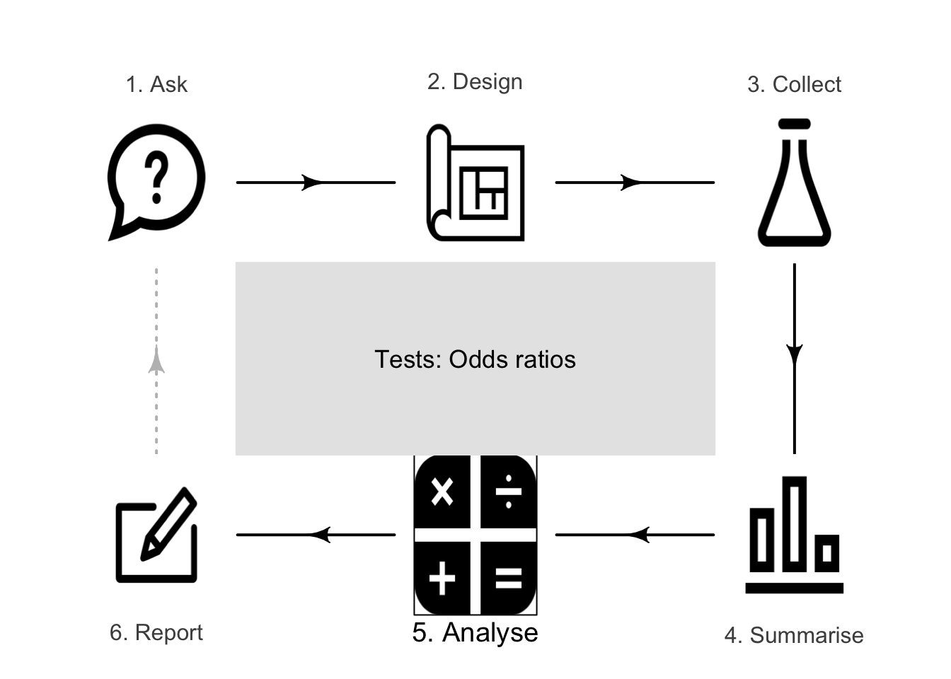
35 Tests comparing qualitative variables

You have learnt to ask a RQ, design a study, classify and summarise the data, construct confidence intervals, and perform some hypothesis tests. In this chapter, you will learn to:

• identify situations where conducting a test for comparing two odds is appropriate.
• conduct hypothesis tests for an OR (i.e., comparing two proportions, or comparing two odds), using chi-square tests in software output.
• determine whether the conditions for using these methods apply in a given situation.

35.1 Introduction: meals on-campus

As seen in Sect. 28.1, Mann and Blotnicky (2017) examined the relationship between where university students usually ate, and where the student lived (Table 35.1).

TABLE 35.1: Where university students live and eat

	Most off-campus	Most on-campus
Living with parents	\(52\)	\(\phantom{0}\phantom{0}2\)
Not living with parents	\(105\)	\(\phantom{0}24\)

A graphical summary is shown in Fig. 28.1 (left panel), and a numerical summary in Table 35.2. (The details of the computations appear in Sect. 28.2).

TABLE 35.2: The odds and percentage of university students eating most meals off-campus

	Odds of having most meals off-campus	Percentage having most meals off-campus	Sample size
Living with parents	\(26.000\)	\(96.3\)	\(\phantom{0}54\)
Not living with parents	\(\phantom{-}4.375\)	\(81.4\)	\(129\)
	\(\phantom{-}5.943\)	\(14.9\)

The parameter can be either a difference between two population proportions, or a population odds ratio. For example, the parameter could be difference between population proportion students of eating most meals off-campus, comparing students living with their parents, to students not living with their parents. Alternatively (and equivalently), the parameter could be the population OR of odds of eating most meals off-campus, comparing students living with their parents, to students not living with their parents.

The table can be constructed with either variable as the rows or the columns. However, software commonly compares rows, so it makes sense to place the groups to be compared (i.e., the explanatory variable) in the rows of the table.

Then, the difference between the two proportions are usually calculated as the Row 1 proportion minus the Row 2 proportion. Similarly, the odds then can be interpreted as comparing Column 1 counts to Column 2 counts, and the odds ratio as comparing the Row 1 odds to the Row 2 odds.

The RQ and the hypotheses can be written as comparing proportions (Sect. 35.2), comparing odds (Sect. 35.3), or about odds ratios. Means are not appropriate (the data contain two qualitative variables).

Since two groups are being compared, subscripts are used to distinguish between the statistics for the two groups; say, Groups \(A\) and \(B\) in general (Table 35.3).

TABLE 35.3: Notation used to distinguish between the two independent groups

	Group A	Group B	Comparing groups
Sample sizes:	\(n_A\)	\(n_B\)
Sample odds:	\(\text{Odds}_A\)	\(\text{Odds}_B\)	\(\text{Odds ratio} = \text{Odds}_A/\text{Odds}_B\)
Sample proportions:	\(\hat{p}_A\)	\(\hat{p}_B\)	\(\hat{p}_A - \hat{p}_B\)
Standard errors:	\(\displaystyle\text{s.e.}(\hat{p}_A)\)	\(\displaystyle\text{s.e.}(\hat{p}_B)\)	\(\displaystyle\text{s.e.}(\hat{p}_A - \hat{p}_B)\)

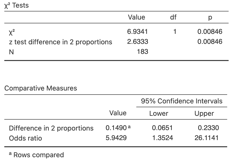
FIGURE 35.1: Software output for computing a CI and conducting a test

35.2 Comparing two proportions: \(z\)-test

To compare the two proportions, the two-tailed RQ is:

Is the population proportion of students eating most meals off-campus the same for students living with their parents and for students not living with their parents?

We use \(N\) to refer to students not living with their parents, ad \(L\) for students living with their parents. Then, following Table 35.3, the parameter in the RQ is the difference between population means: \(p_L - p_N\). As usual, the population values are unknown, so this is estimated using the statistic \(\hat{p}_L - \hat{p}_N\).

Hypothesis testing always begins by assuming that the null hypothesis is true (Sect. 32.2.1). In this context, that means assuming that the population proportion of eating most meals off-campus is the same in both groups. As a result, the data from the two groups can be combined to determine an overall (or common) proportion of students eating most meals off-campus: \[ \hat{p} = \frac{52 + 105}{52 + 105 + 2 + 24} = \frac{157}{183} = 0.85792. \] This is the overall proportion of students eating most meals off-campus, assuming no difference between students living with and not with their parents.

The two sample proportions will vary from sample to sample and so have a sampling distribution (as in Sect. 30.3). The standard error of \(\hat{p}\) for each sample is computed using this common proportion, using the same idea as in Eq. (23.2):
\[\begin{align*} \text{s.e.}(p_L) &= \sqrt{ \frac{p\times(1 - p)}{n_L}} = \sqrt{ \frac{0.85792\times(1 - 0.85792)}{54}} = 0.047511; \text{and}\\ \text{s.e.}(p_N) &= \sqrt{ \frac{p\times(1 - p)}{n_N}} = \sqrt{ \frac{0.85792\times(1 - 0.85792)}{129}} = 0.030739. \end{align*}\] The difference between the proportions will vary from sample to sample too, and hence have a sampling distribution. The standard error of this sampling distribution for the difference between the proportions is \[ \text{s.e.}(\hat{p}_A - \hat{p}_B) = \sqrt{ \text{s.e.}(\hat{p}_L)^2 + \text{s.e.}(\hat{p}_N)^2 } = \sqrt{ 0.047511^2 + 0.030739^2} = 0.056588, \] similar to Eq. (28.1).

Definition 35.1 (Sampling distribution for the difference between two sample proportions) The sampling distribution of the difference between two sample proportions \(\hat{p}_A\) and \(\hat{p}_B\) is (when the appropriate conditions are met; Sect. 35.4) described by:

• an approximate normal distribution,
• centred around a sampling mean whose value is \({p_{A}} - {p_{B}}\), the difference between the population proportions (from \(H_0\)),
• with a standard deviation, called the standard error of the difference between the proportions, of \(\displaystyle\text{s.e.}(\hat{p}_A - \hat{p}_B)\).

The standard error for the difference between the proportions is \[ \text{s.e.}(\hat{p}_A - \hat{p}_B) = \sqrt{ \text{s.e.}(\hat{p}_A)^2 + \text{s.e.}(\hat{p}_B)^2 }, \] where \[ \text{s.e.}(p_A) = \sqrt{ \frac{p\times(1 - p)}{n_A}} \quad\text{and}\quad \text{s.e.}(p_B) = \sqrt{ \frac{p\times(1 - p)}{n_B}} \] where \(p\) is the common (overall) proportion.

Since the sampling distribution has an approximate normal distribution, the test statistic is \[ z = \frac{ (\hat{p}_L - \hat{p}_N) - (p_L - p_N) }{\text{s.e.}(\hat{p}_A - \hat{p}_B)} \ = \frac{ 0.14901 - 0}{0.056588} = 2.633 \] Since the test-statistic is a \(z\)-score, the \(P\)-value can be computed from normal distributions (Sect. 21.6) or from software output (Fig. 35.1). The two-tailed \(P\)-value reported by software (Fig. 35.1, under the column p) is indeed small: \(0.008\) to three decimals.

A very small \(P\)-value (\(0.008\) to three decimals) means strong evidence exists to supporting \(H_1\): the evidence suggests a difference between the population proportions. We write:

The sample provides strong evidence (\(z = 2.63\); two-tailed \(P = 0.008\)) that the proportion of students in the population of having most meals off-campus is different for students living with their parents (proportion: \(0.963\)) and students not living with their parents (proportion: \(0.814\); difference: \(0.149\); \(95\)% CI from \(0.0633\) and \(0.235\), higher for students living with their parents).

The conclusion includes three components (Sect. 32.8): the answer to the RQ; the evidence used to reach that conclusion ('\(z = 2.63\); two-tailed \(P = 0.008\)'); and some sample summary statistics (including the \(95\)% CI for the difference between proportions).

The conclusion also makes clear which proportion is higher.

35.3 Comparing two odds: \(\chi^2\)-test

For the \(2\times 2\) table of counts in Table 35.1, odds can be compared rather than proportions:

Are the population odds of students eating most meals off-campus the same for students living with their parents and for students not living with their parents?

If the odds are the same in the two groups, this is equivalent to an odds ratio of one. Hence, the RQ could also be written as

Is the population odds ratio of eating most meals off-campus, comparing students who live with their parents to students not living with their parents, equal to one?

Either way, the parameter is the population odds ratio, and the null hypothesis is the 'no difference, no change, no relationship' position:

• \(H_0\): The population OR is one; or (equivalently):
  The population odds are the same in each group.

This hypothesis proposes that the sample odds are not the same in the two groups only due to sampling variation. This is the initial assumption. The alternative hypothesis is

• \(H_1\): The population OR is not one; or (equivalently):
  The population odds are not the same in each group.

For comparing odds, the alternative hypotheses is always two-tailed.

In our example then:

• \(H_0\): The population odds of eating most meals off-campus are the same for students living with their parents and for students not living with their parents.
• \(H_1\): The population odds of eating most meals off-campus are different for students living with their parents and for students not living with their parents.

As usual, the decision-making process starts by assuming the null hypothesis is true: that the population odds ratio is one (i.e., the population odds in each group are equal).

35.3.1 Finding expected counts

Assuming that the odds of having most meals off-campus is the same for both groups (that is, the population OR is one), how would the sample OR be expected to vary from sample to sample just because of sampling variation? If the null hypothesis is true, the odds are the same in both groups (and the proportions are the same in both groups). That is, the proportions of students eating most meals off-campus is the same for students living with and not living with their parents.

Let's consider the implication. From Table 35.1, \(157\) students out of \(183\) ate most meals off-campus, so that \(157\div 183 = 0.8579\) of students in the entire sample ate most of their meals off-campus.

If the proportions of students who eat most of their meals off-campus is the same for those who live with their parents and those who don't, then we'd expect \(0.8579\) of students in both groups to be eating most meals off-campus. (These values were also found in Sect. 28.5.) In other words, the two conditional probabilities would be the same. In that case, we would expect:

• A proportion of \(0.8579\) of the \(54\) students who live with their parents (i.e., \(46.33\) students) to eat most meals off-campus; and
• A proportion of \(0.8579\) of the \(129\) students who don't live with their parents (i.e., \(110.67\) students) to eat most meals off-campus.

In other words, the proportions (and hence the odds) of eating most meals off-campus is the same in each group. Those are the expected counts if the proportions (or odds) was exactly the same in each group (Table 35.4), if the null hypothesis (the assumption) was true.

How close are the observed counts (Table 35.1) to the expected counts (Table 35.4)?

• \(46.33\) of the \(54\) students who live with their parents are expected to eat most meals off-campus; yet we observed \(52\).
• \(110.67\) of the \(129\) students who don't live with their parents are expected to eat most meals off-campus; yet we observed \(105\).

The observed and expected counts are similar, but not the exactly same. The difference between the observed and expected counts may be explained by sampling variation (that is, the null hypothesis explanation).

You do not have to compute the expected values when you answer one of these types of RQs (software does it in the background). However, seeing how the decision-making process works in this context is helpful.

In previous hypothesis tests, the sampling distribution had an approximate normal distribution. However, the sampling distribution of the odds ratio is more complicated¹¹ so will not be presented. We will use software output to conduct the test.

TABLE 35.4: Where university students live and eat: expected counts

	Most off-campus	Most on-campus	Total
Living with parents	\(46.328\)	\(\phantom{0}\phantom{0}7.672\)	\(\phantom{0}54\)
Not living with parents	\(110.672\)	\(\phantom{0}18.328\)	\(129\)
Total	\(157.000\)	\(\phantom{0}26.000\)	\(183\)

35.3.2 Computing the value of the test statistic

The decision-making process compares what is expected if the null hypothesis about the parameter is true (Table 35.4) to what is observed in the sample (Table 35.1). Previously, when the summary statistics were means and the sampling distribution was a normal distribution, the test statistic was a \(t\)-score. However, the data here are not summarised by means, the sampling distribution is not a normal distribution (but is related to a normal distribution), and so a different test statistic is needed.

Here, the test-statistic is a 'chi-squared' statistic, written \(\chi^2\). The \(\chi^2\)-score measures the overall size of the differences between the expected counts and observed counts, over the entire \(2\times 2\) table.

The Greek letter \(\chi\) is pronounced 'ki', as in kite (not 'chi' as in China). The test statistic \(\chi^2\) is pronounced as 'chi-squared'.

From the software (Fig. 35.1), \(\chi^2 = 6.934\). But what does this value mean? Is it 'large' or 'small'?

The \(\chi^2\)-value can be understood by finding the equivalent \(z\)-score, which means a \(P\)-value can be estimated using the \(68\)--\(95\)--\(99.7\) rule. The \(\chi^2\)-value is equivalent to \[ z = \sqrt{\chi^2}\qquad\text{for a $2\times 2$ table}. \] Here, the \(\chi^2\) value is equivalent to a \(z\)-score of \(\sqrt{6.934} = 2.633\). This is the same \(z\)-score produced when comparing two proportions (Sec. 35.2; Fig. 35.1), and hence the \(P\)-value will be the same also. Using the \(68\)--\(95\)--\(99.7\) rule, a small \(P\)-value is expected. The two-tailed \(P\)-value reported by software (Fig. 35.1, under the column p) is indeed small: \(0.008\) to three decimals.

Recall that, for two-way tables of counts, the alternative hypotheses are always two-tailed, so a two-tailed \(P\)-value is always reported.

Click on the hotspots in the following image, and describe what the software output tells us.

35.3.3 Writing conclusions

A very small \(P\)-value (\(0.008\) to three decimals) means strong evidence exists to supporting \(H_1\): the evidence suggests a difference in the population odds in the two groups. We write:

The sample provides strong evidence (\(\chi^2 = 6.934\); two-tailed \(P = 0.008\)) that the odds in the population of having most meals off-campus is different for students living with their parents (odds: \(26\)) and students not living with their parents (odds: \(4.375\); OR: \(5.94\); \(95\)% CI from \(1.35\) to \(26.1\)).

The conclusion includes three components (Sect. 32.8): The answer to the RQ; the evidence used to reach that conclusion ('\(\chi^2 = 6.934\); two-tailed \(P = 0.008\)'); and some sample summary statistics (including the \(95\)% CI for the odds ratio).

The conclusion also makes clear what the odds and the odds ratio mean. The odds are describing as the 'odds... of having most meals off-campus', and the OR as then comparing these odds between 'students living with their parents... and students not living with their parents'.

For two-way tables, RQs are best framed in terms of ORs or comparing odds (but can be framed in terms of proportions or percentages, or associations or relationships). Usually, RQs are easiest to write when framed in terms of comparing odds.

For consistency: if the RQ is about the odds ratio, the hypotheses and conclusion should be about the odds ratio; if the RQ is about odds, the hypotheses and conclusion should be about the odds; and so on.

35.4 Statistical validity conditions

As usual, these results hold under certain conditions. The test above is statistically valid if:

• All expected counts are at least five.

Some books may give other (but similar) conditions.

The statistical validity condition refers to the expected (not the observed) counts. In some software, the expected counts must be explicitly requested to see if this condition is satisfied (Fig. 35.2).

If all the observed counts exceed five, then all expected counts will exceed five.

The units of analysis are also assumed to be independent (e.g., from a simple random sample).

If the statistical validity conditions are not met, other similar options include using a Fisher's exact test (Conover 2003) or using resampling methods (Efron and Hastie 2021).

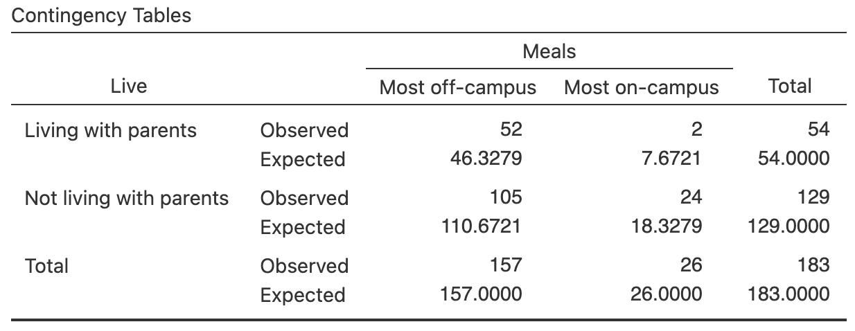
FIGURE 35.2: The expected values, as computed by software

For the student-eating data, the smallest observed count is \(2\) (living with parents; most meals off-campus), but the smallest expected count is \(7.67\), which is greater than five. The size of the expected counts is important for the statistical validity condition.

Example 35.1 (Statistical validity) For the university-student eating data, all the cells have an expected count of at least five so the statistical validity condition is satisfied.

35.5 Tests of independence more generally: \(\chi^2\)-tests

Often a tables of counts is larger than \(2\times 2\). In these situations, the RQ is worded in terms of independence, relationships or associations (but not correlations) between the variables:

Is there a relationship (or association) between one qualitative variable and another qualitative variable?

The RQ is answered using a \(\chi^2\)-test comparing odds (not proportions), by extending the ideas in Sect. 35.3, as demonstrated in the following example.

Example 35.2 (Larger two-way tables) [Dataset: RipsID] Diez-Fernández et al. (2023) studied Spanish people's knowledge of ocean rips (Table 35.5, left table). The table is a \(4\times 2\) two-way table. The RQ is

Is there a relationship (or association) between age group and people's ability to correctly identify a rip?

TABLE 35.5: Identifying rips. Left: the data by age group. Right: a summary table. The odds ratio is relative to the 51 to 65 age group.

	Correctly	Incorrectly
18 to 24	\(\phantom{0}41\)	\(\phantom{0}5\)
25 to 34	\(\phantom{0}47\)	\(12\)
35 to 50	\(106\)	\(19\)
51 to 65	\(\phantom{0}52\)	\(\phantom{0}7\)

The odds and percentage of people in each age group that can correctly identify rips can be computed (Table 35.5, right table), but this is not always possible (e.g., for a \(3\times 4\) table). Odds ratios compare pairs of odds, so the odds ratios in Table 35.5 are all relative to those \(51\) to \(65\) (hence, no odds ratio is given for the \(51\) to \(65\) age group, which is the reference level). For example, the odds of someone aged \(18\) to \(24\) correctly identifying a rip is \(1.104\) times the odds of someone aged \(51\) to \(65\) correctly identifying a rip.

• \(H_0\): In the population, there is no association between age group and being able to correctly identify a rip;
• \(H_1\): In the population, there is an association between age group and being able to correctly identify a rip.

For a \(2\times 2\) table, the parameter is the odds ratio, and the test proceeds using a \(\chi^2\) value. As in Sect. 35.3, the value of \(\chi^2\) compares the observed counts to the expected counts (found in the same way as in Sect. 35.3.1). For two-way tables larger than \(2\times 2\), defining a single parameter to describe the association between the variables is difficult.

When no relationship exists in the sample, the observed and expected values are the same, and \(\chi^2 = 0\). The larger the difference between the observed and expected values, the larger the value of \(\chi^2\). Sampling variation means that the observed values will vary from sample to sample, so that \(\chi^2\) may not be exactly zero, even if there is no association between the variables.

Software computes \(\chi^2 = 2.4062\) (Fig. 35.3). For two-way table of counts larger than \(2\times 2\), this is equivalent to a \(z\)-score of \[ z = \sqrt{\chi^2 \div \text{df}}, \] where \(\text{df}\) is the degrees of freedom, where \[ \text{df} = (\text{number of columns of data} - 1)\times(\text{number of rows of data} - 1). \] Here, \(\text{df} = (4 - 1)\times ( 2 - 1) = 3\), as in the output (Fig. 35.3). Hence, the equivalent \(z\)-score is \[ z = \sqrt{2.4062/3} = 0.896, \] which is quite small, so we expected a large \(P\)-value. Software confirms this (Fig. 35.3): \(P = 0.492\).

Recall that, for two-way tables of counts, the alternative hypotheses are always two-tailed, so a two-tailed \(P\)-value is always reported.

In a chi-squared test, the value of \[ \sqrt{ \chi^2 \div {\text{df}}} \] is like a \(z\)-score, where \(\text{df}\) is the 'degrees of freedom' (df in the software output). The degrees of freedom in a two-way table is the number of rows of data less one, times the number of columns of data less one.

This allows the \(P\)-value to be estimated using the \(68\)--\(95\)--\(99.7\) rule.

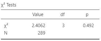
FIGURE 35.3: Software output for the hypothesis test about knowledge of ocean rips

The statistical validity conditions are the same as in Sect. 35.4: all expected counts are at least five.

Click on the hotspots in the following image, and describe what the jamovi output tells us.

35.6 Example: turtle nests

(This study was seen in Sect. 28.6.) The hatching success of loggerhead turtles on Mediterranean beaches is often compromised by fungi and bacteria. Candan, Katılmış, and Ergin (2021) compared the odds of a nest being infected, between nest relocated due to the risk of tidal inundation, and non-relocated nests (Table 35.6). The researchers were interested in knowing:

For Mediterranean loggerhead turtles, are the odds of infections the same for natural and relocated nests?

TABLE 35.6: Infected and non-infected turtle nests

	Non-infected	Infected
Natural	\(29\)	\(10\)
Relocated	\(14\)	\(\phantom{0}8\)

The parameter is the odds ratio of infection, comparing natural to relocated nests. A graphical summary is shown in Fig. 28.3. A numerical summary table (Table 28.3, right table) shows that the odds of natural nest being infected is \(1.657\) times the odds of a relocated nest being infected. From the software output (Fig. 35.4), the \(\chi^2\)-value is \(0.777\). This is like a \(z\)-score of \(z = \sqrt{0.777/1} = 0.88\), which is very small, so expect a large \(P\)-value. Indeed, the \(P\)-value is \(0.378\) on the output. The smallest expected count is \(6.49\) (Fig. 35.4), so this test is statistically valid. We write:

There is no evidence of a difference in the odds of infection (\(\chi^2\): \(0.777\); \(P\)-value: \(0.378\); odds ratio: \(1.657\); \(95\)% CI: \(0.537\) to \(5.12\)) between natural nests (odds: \(2.90\); \(n = 39\)) and relocated nests (odds: \(1.75\); \(n = 22\)).

That is, there no evidence that relocating the nest (to protect them from tidal inundation) changes the risk of infection.

We do not say whether the evidence supports the null hypothesis. We assume the null hypothesis is true, so we state how strong the evidence is to support the alternative hypothesis. The current sample presents no evidence to contradict the assumption, but future evidence may emerge.

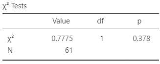
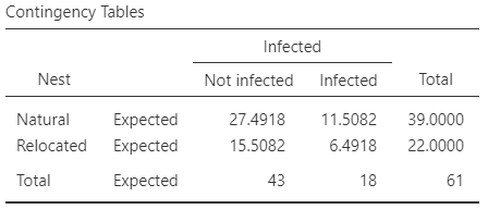
FIGURE 35.4: The software output for the turtle-nesting data

35.7 Example: shopping bags

A study of \(400\) residents of Klang Valley, Malaysia, examined residents' approach to waste management (Choon, Tan, and Chong 2017). One RQ was:

For residents of Klang Valley, is age group associated with whether people bring their own bags when shopping?

The data (Table 35.7) are given in a \(3\times 2\) table of counts. The software output is shown in Fig. 35.5, and a graphical summary in Fig. 35.6.

TABLE 35.7: Whether shoppers bring their own bags, and the shoppers age

	Brings own bags	Does not bring own bags
30 and under	\(126\)	\(138\)
31 to 40	\(\phantom{0}50\)	\(\phantom{0}32\)
Over 40	\(\phantom{0}41\)	\(\phantom{0}13\)

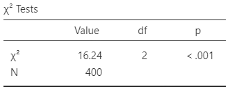
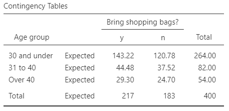
FIGURE 35.5: Software output for the shopping-bags data

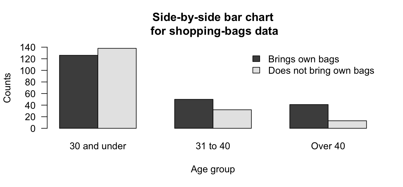
FIGURE 35.6: A side-by-side bar chart for the shopping-bags data

TABLE 35.8: Odds and percentage that people bring their own shopping bags by age groups. The odds ratios are computed relative to those 'Over \(40\)'.

	Odds	Odds ratio	Percentage	Sample size
30 and under	\(0.913\)	\(0.289\)	\(47.7\)	\(264\)
31 to 40	\(1.563\)	\(0.496\)	\(61.0\)	\(\phantom{0}82\)
Over 40	\(3.154\)		\(75.9\)	\(\phantom{0}54\)

For the numerical summary table (Table 35.8):

• For those '\(30\) or under': the odds of bringing a shopping bag is \(126/138 = 0.913\).
• For those '\(31\) to \(40\)': the odds of bringing a shopping bag is \(50/32 = 1.563\).
• For those 'Over \(40\)': the odds of bringing a shopping bag is \(41/13 = 3.154\).

For computing the odds ratios, Row 3 is on the bottom of the fraction (as the reference level):

• The OR of bringing a shopping bag, comparing people '\(30\) and under' to people 'Over \(40\)': \(0.913/3.154 = 0.289\).
• The OR of bringing a shopping bag, comparing people '\(31\)--\(40\)' to people 'Over \(40\)': \(1.563/3.154 = 0.496\).

That is, the odds of bringing a shopping bag for those '\(30\) and under' is \(0.289\) times (i.e., is smaller than) the odds of those 'Over \(40\)'. Similarly, the odds of bringing a shopping bag for those '\(31\) to \(40\)' is \(0.496\) times (i.e., is smaller than) the odds of those 'Over \(40\)'.

The hypothesis can be worded in terms of odds, but the hypothesis are usually worded in terms of associations (but not correlations) for tables larger than \(2\times 2\):

• \(H_0\): No association exists between bringing a shopping bag and age group.
• \(H_1\): An association exists between bringing a shopping bag and age group.

From the software output (Fig. 35.5), \(\chi^2 = 16.24\) and \(\text{df} = 2\), so this \(\chi^2\) value is approximately equivalent to a \(z\)-score of \(\sqrt{16.24\div 2} = 2.85\). This is a large \(z\)-score so, using the \(68\)--\(95\)--\(99.7\) rule, a small \(P\)-value is expected; indeed, software reports \(P < 0.001\). This suggests very strong evidence in the sample that bringing a shopping bag is not the same for all three age groups.

The conclusion could be written as

The sample provides very strong evidence (\(\chi^2 = 16.24\); \(\text{df} = 2\)) that the odds of bringing a shopping bag is not the same for the three age groups.

Adding sample summary information to this conclusion is cumbersome. Instead, readers can be pointed to the numerical summary (Table 35.8). Furthermore, CIs are not reported since software does not always produce CIs for tables larger than \(2\times 2\).

While we know there is an association between the variables, we can only speculate on the nature of the association (i.e., for which group(s) the population odds are different). Comparing all pairs of groups increases the probability of incorrectly declaring a difference between the odds (increasing the chance of a Type I error; Sect. 32.7) The correct approach requires methods beyond this book.

All expected values exceed \(5\) (Fig. 35.5), so the results are statistically valid.

35.8 Chapter summary

To test a hypothesis about a difference between two population proportions \(p_A - p_B\):

• Write the null hypothesis (\(H_0\)) and the alternative hypothesis (\(H_1\)).
• Initially assume the value of \((p_A - p_B)\) in the null hypothesis to be true.
• Then, describe the sampling distribution, which describes what to expect from the difference between the sample proportions based on this assumption: under certain statistical validity conditions, the difference between the sample proportions vary with:
  • an approximate normal distribution,
  • with sampling mean whose value is the value of \((p_A - p_B)\) (from \(H_0\)), and
  • having a standard deviation of \(\displaystyle \text{s.e.}(\hat{p}_A - \hat{p}_B)\).
• Compute the value of the test statistic: \[ z = \frac{ (\hat{p}_A - \hat{p}_B) - (p_A - p_B)}{\text{s.e.}(\hat{p}_A - \hat{p}_B)}, \] where \(p_A - p_B\) is the hypothesised difference given in the null hypothesis.
• The \(t\)-value is like a \(z\)-score, and so an approximate \(P\)-value can be estimated using the \(68\)--\(95\)--\(99.7\) rule, or found using software.

To test a hypothesis for comparing two odds, or to test for a relationship between two qualitative variables more generally:

• Write the null hypothesis (\(H_0\)) and the alternative hypothesis (\(H_1\)).
• Initially assume no relationship between the two variables.
• Find the value of the test statistic (a \(\chi^2\)-score) on the software output.
• The equivalent \(z\)-score is \(\sqrt{\chi^2\div\text{df}}\) where \(\text{df}\) is the 'degrees of freedom' and can be found on the software output.
• An approximate \(P\)-value can be estimated using the \(68\)--\(95\)--\(99.7\) rule, or found using software.

35.9 Quick review questions

Meresa, Tadesse, and Zeray (2023) investigated Ethiopian farmers' adoption of improved soil and water conservation structures on their farms (Table 35.9). Software output is shown in Fig. 35.7.

TABLE 35.9: Adoption of conservation practices by Etghiopian farmers, by farm size

	Non-adopter	Adopter
\(< 0.5\) ha	\(86\)	\(61\)
\(\ge 0.5\) ha	\(43\)	\(71\)

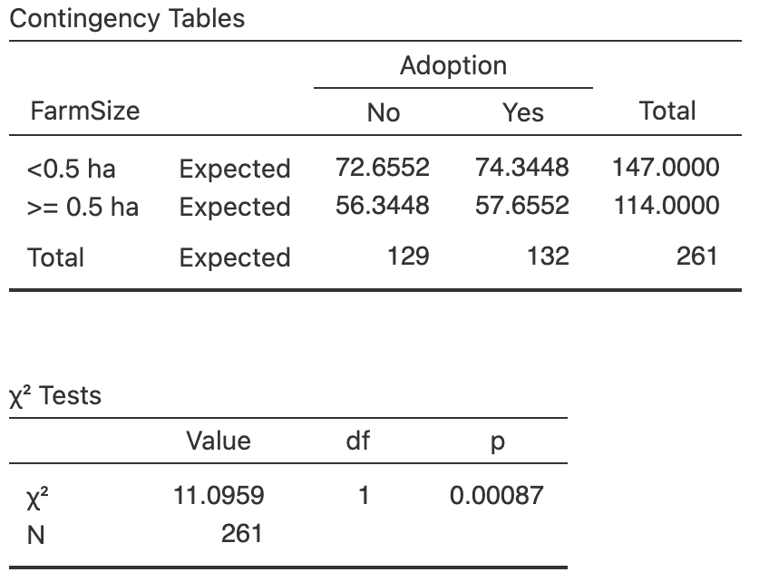
FIGURE 35.7: Software output for the farming study

1. What is the \(\chi^2\) value? 10.7105 2.2903 1.3891 262
2. How many degrees of freedom are there?
3. What is the equivalent \(z\)-score (to two decimal places)?
4. Using the \(68\)--\(95\)--\(99.7\) rule, what is the approximate \(P\)-value?
   Smaller than 0.003Smaller than 0.05Larger than 0.05There is not enough information
5. From the software output, what is the \(P\)-value? 10.7105 0.00107 2.2903 There is not enough information
6. Is the alternative hypothesis one- or two-tailed?
   One-tailedTwo-tailedThere is not enough information
7. True or false: There is no evidence of a difference in odds of adopting of conservation practices, for the two far size categories. TRUE FALSE
8. True or false: The test will be statistically valid. TRUE FALSE

35.10 Exercises

Answers to odd-numbered exercises are available in App. E.

Exercise 35.1 Consider the expected counts in Table 35.4. Confirm that the odds of having most meals off-campus is the same for students living with their parents, and for students not living with their parents.

Exercise 35.2 Consider the expected counts in Fig. 35.7. Confirm that the odds of being an adopter of improved soil and water conservation structures is the same for smaller and larger farms.

Exercise 35.3 Christensen, Herrer, and Telford (1972) studied the number of sandflies caught in light traps set at \(3\) and \(35\) feet above ground in eastern Panama. They asked:

In eastern Panama, are the odds of finding a male sandfly the same at \(3\) feet above ground as at \(35\) feet above ground?

The data are compiled into a table (Table 35.10), and summarised numerically (Table 35.11; partially edited) and graphically (Fig. 35.8). Use the software output (Fig. 35.9) to evaluate the evidence, complete Table 35.11, and write a conclusion.

TABLE 35.10: The sex of sandflies at two heights

	3 feet	35 feet
	Males	Females
Males	\(173\)	\(125\)
Females	\(150\)	\(\phantom{0}73\)

TABLE 35.11: Odds and percentages of male sandflies at two heights above ground level

	Odds	Percentage	Sample size
3 feet above ground:			\(298\)
35 feet above ground:	\(1.71\)	\(67.3\)	\(223\)
Odds ratio:	\(0.67\)

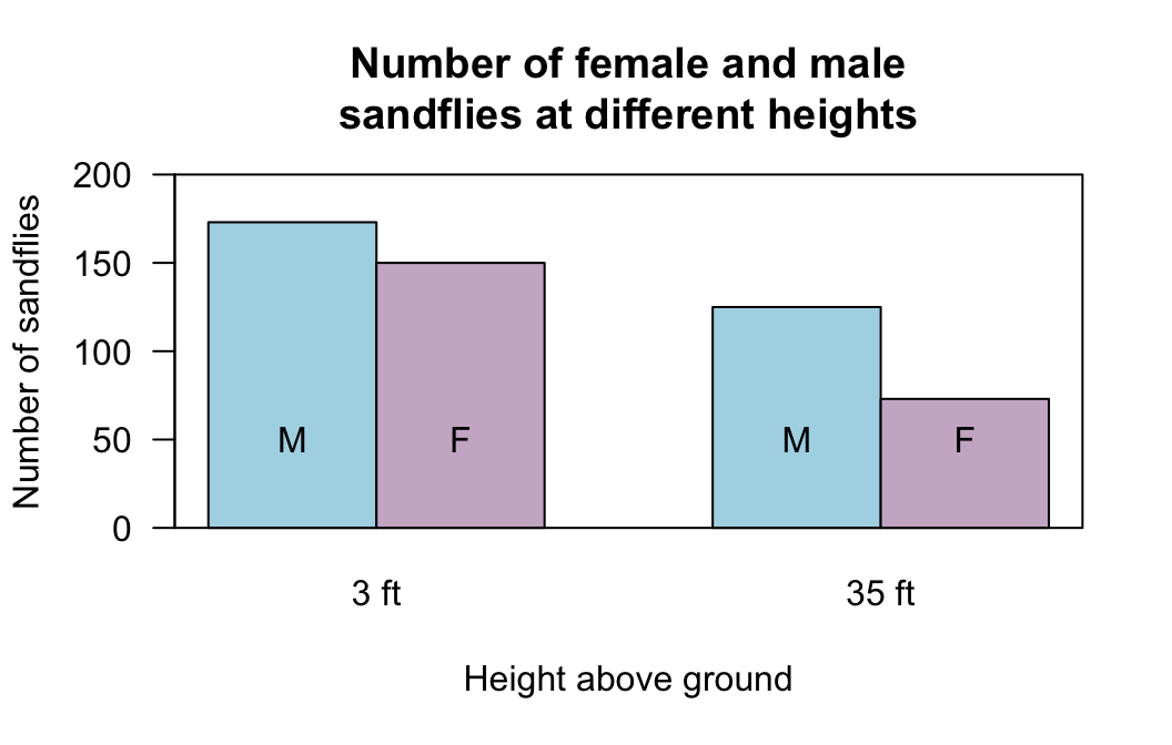
FIGURE 35.8: A side-by-side barchart of the sandflies data

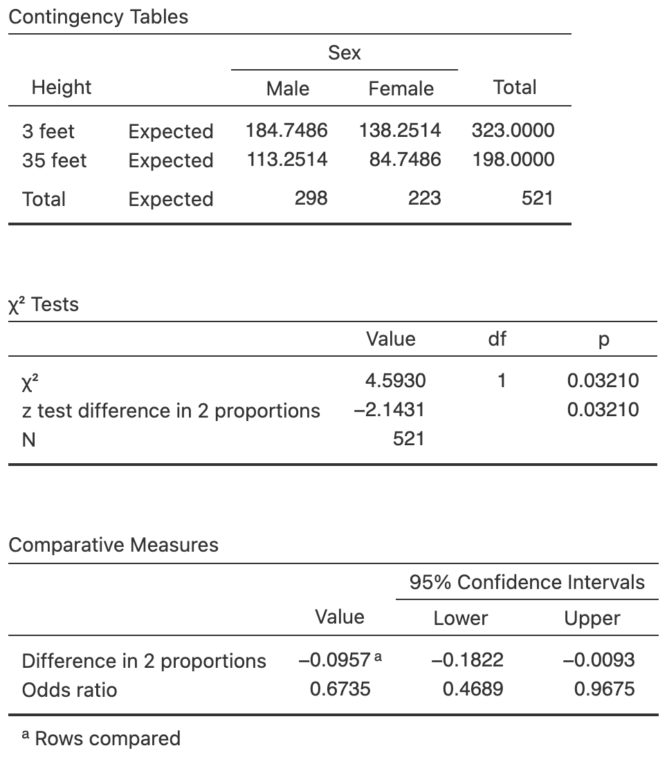
FIGURE 35.9: Software output for the sandflies data

Exercise 35.4 (This study also appeared in Exercise 28.4, where the odds ratio, and the CI for the odds ratio, were computed.) Wallace et al. (2017) compared the heights of scars from burns received in Western Australia (Table 28.7). The data are shown in Table 35.12. Software was used to analyse the data (Fig. 35.10).

1. Perform a hypothesis test to determine if the odds of having a smooth scar are the same for women and men.
2. Write down the conclusion.
3. Is the test statistically valid?

TABLE 35.12: The number of men and women, with scars of different heights

	\(0\) mm (smooth)	Between \(0\) mm and \(1\) mm
Women	\(99\)	\(\phantom{0}62\)
Men	\(216\)	\(115\)

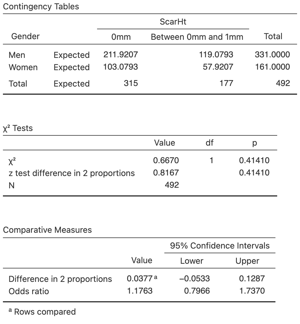
FIGURE 35.10: Software output for the scar-height data

Exercise 35.5 A study of turbine failures (Myers, Montgomery, and Vining 2002; Nelson 1982) ran \(73\) turbines for around \(1800\) hrs, and found that seven developed fissures (small cracks). They also ran a different set of \(42\) turbines for about \(3000\) hrs, and found that nine developed fissures.

1. Use the software output (Fig. 35.11, left panel) to test for a relationship.
2. Compute, then carefully interpret, the OR.
3. Write down, then carefully interpret, the test results.
4. Is the CI statistically valid (Fig. 35.11, right panel)?

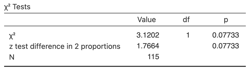
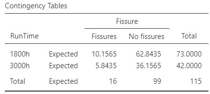
FIGURE 35.11: Software output for the turbine data (left); expected counts (right)

Exercise 35.6 (This study also appeared in Exercise 28.7.) The Southern Oscillation Index (SOI) is a standardised measure of the air pressure difference between Tahiti and Darwin, and has been shown to be related to rainfall in some parts of the world (Stone, Hammer, and Marcussen 1996), and especially Queensland (Stone and Auliciems 1992).

The rainfall at Emerald (Queensland) was recorded for Augusts between 1889 to 2002 inclusive (P. K. Dunn and Smyth 2018), where the monthly average SOI was positive, and when the SOI was non-positive (that is, zero or negative), as shown in Table 35.13.

1. Using the software output in Fig. 35.12, perform a hypothesis test to determine if the odds of having no rain is the same Augusts with non-positive and negative SOI.
2. Write down the conclusion.
3. Is the test statistically valid?

TABLE 35.13: The SOI, and whether rainfall was recorded in Augusts between 1889 and 2002 inclusive

	Rainfall recorded	No rainfall recorded
Positive SOI	\(53\)	\(\phantom{0}7\)
Non-positive SOI	\(40\)	\(14\)

FIGURE 35.12: Software output for the Emerald-rain data

Exercise 35.7 [Dataset: HatSunglasses] (This study also appeared in Exercise 28.8.) B. Dexter et al. (2019) recorded the number of people at the foot of the Goodwill Bridge, Brisbane, who wore hats between \(11\):\(30\)am to \(12\):\(30\)pm. Of the \(386\) males observed, \(79\) wore hats; of the \(366\) females observed, \(22\) wore hats.

1. Compute the percentages of females wearing a hat.
2. Compute the percentages of males wearing a hat.
3. Compute the odds of a female wearing a hat.
4. Compute the odds of a male wearing a hat.
5. Compute the odds ratio of wearing a hat, comparing females to males.
6. Compute the odds ratio of wearing a hat, comparing males to females.
7. Find the \(95\)% CI for the appropriate OR.
8. Using the software output in Fig. 35.13, perform a hypothesis test to determine if the odds of wearing a hat is the same for females and males.
9. Write down the conclusion.
10. Is the test statistically valid?

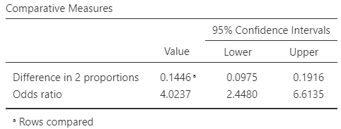
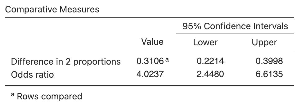
FIGURE 35.13: Software output for the hats data

Exercise 35.8 Witmer and Pipas (2020) compared various types of repellents to stop bears damaging trees in an Idaho forest. Part of the data are summarised in Table 35.14.

1. Compute the column percentages.
2. Compute the odds of new damage for both repellents.
3. Compute the proportion of trees with new damage.
4. Compute the odds ratio, and the difference between the proportions.
5. Write the hypothesis for conducting a hypothesis test.
6. Compute the expected counts.
7. Software gives \(\chi^2\) is \(4.4850\). What is the approximately-equivalent \(z\)-score? Would you expect a large or small \(P\)-value?
8. The \(P\)-value is given as \(P = 0.0342\). Write a conclusion.

TABLE 35.14: The number of trees with new damage by bears, according to different repellents

	New damage
	Yes	No
Bear faeces	\(\phantom{0}6\)	\(69\)
Control (water)	\(15\)	\(60\)

Exercise 35.9 [Dataset: PetBirds] (This study also appeared in Exercise 28.9.) Kohlmeier et al. (1992) examined people with lung cancer, and a matched set of controls who did not have lung cancer, and recorded the number in each group that kept pet birds. The data are shown again in Table 35.15.

Consider this RQ:

Are the odds of having a pet bird the same for people with lung cancer (cases) and for people without lung cancer (controls)?

1. Carefully describe the parameter.
2. Write the hypotheses in terms of odds.
3. Determine the value of \(z\) that is approximately the same as this \(\chi^2\)-value.
4. Use the software output to conduct a hypothesis test.

TABLE 35.15: The pet bird data

	Adults with lung cancer	Adults without lung cancer	Total
Did not keep pet birds	\(141\)	\(328\)	\(469\)
Kept pet birds	\(\phantom{0}98\)	\(101\)	\(199\)
Total	\(239\)	\(429\)	\(668\)

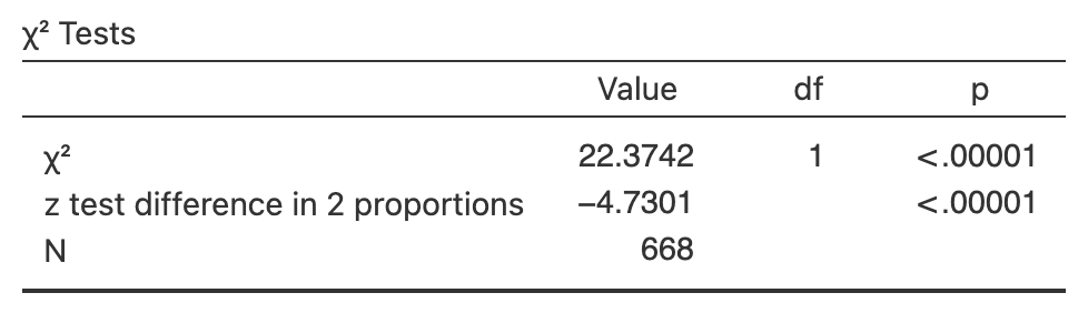
FIGURE 35.14: Software output for the pet-birds data

Exercise 35.10 [Dataset: B12Long] (This study was seen in Exercise 28.10.) Gammon et al. (2012) examined B12 deficiencies in 'predominantly overweight/obese women of South Asian origin living in Auckland', some of whom were on a vegetarian diet and some of whom were on a non-vegetarian diet. One RQ was:

Among a certain group of women, are the odds of being vitamin B12 deficient different for women on a vegetarian diet compared to women on a non-vegetarian diet?

The data are shown in Table 28.10.

1. Write down the hypotheses in terms of odds.
2. Write down the parameter.
3. Determine the \(\chi^2\) value and perform a hypothesis to answer the RQ, using the output in Fig. 35.15.
4. Compute the equivalent \(z\)-score for this \(\chi^2\)-value.
5. Write down the conclusion.
6. Is the test statistically valid?

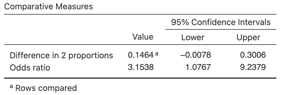
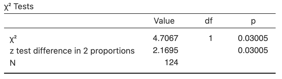
FIGURE 35.15: Software output for the B12 data

Exercise 35.11 [Dataset: DogWalks] Naughton, Grzelak, and Naughton (2024) studied the difference between dogs kept in the city and on farms. One RQ was:

For Northern Ireland dogs, is there an association between length of dog walks, and their location?

The data are shown in Table 35.16.

1. Write down the hypotheses.
2. Determine the \(\chi^2\) value and perform a hypothesis to answer the RQ, using the output in Fig. 35.16.
3. Determine the number of degrees freedom.
4. Compute the equivalent \(z\)-score for this \(\chi^2\)-value.
5. Write down the conclusion.
6. Is the test statistically valid?

TABLE 35.16: The length of walks for dogs, living in the city and farms. ('Varies' means usuually short walks, but occasional longer walks.)

	Walk length (in mins)
	Under \(30\)	\(30\) to under \(60\)	\(60\) to under \(120\)	Varies
City	\(138\)	\(\phantom{0}84\)	\(\phantom{0}13\)	\(264\)
Farm	\(\phantom{0}84\)	\(102\)	\(\phantom{0}33\)	\(243\)

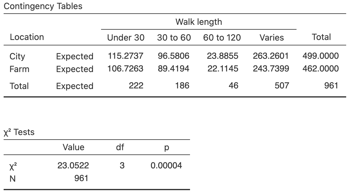
FIGURE 35.16: Software output for the dog-walking data

Exercise 35.12 [Dataset: Mumps] Soud et al. (2009) studied the compliance of students with an isolation request following a large mumps outbreak in Kansas in 2006. One RQ was:

Is there an association between age group, and compliance with the isolation order?

The data are shown in Table 35.17.

1. Write down the hypotheses.
2. Compute the proportion of each age group that complied with the isolation request.
3. Compute the odds of each age group that complied with the isolation request.
4. Compute the relevant odds ratios, and interpret what these mean.
5. Determine the \(\chi^2\) value and perform a hypothesis to answer the RQ, using the output in Fig. 35.17.
6. Determine the number of degrees freedom.
7. Compute the equivalent \(z\)-score for this \(\chi^2\)-value.
8. Write down the conclusion.
9. Is the test statistically valid?

TABLE 35.17: The compliance of students by age group

	Compliance
	Yes	No
\(18\) to \(19\)	\(40\)	\(10\)
\(20\) to \(21\)	\(37\)	\(14\)
Older than \(22\)	\(22\)	\(\phantom{0}9\)

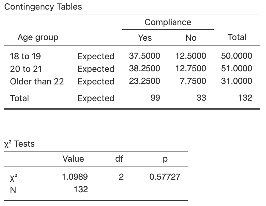
FIGURE 35.17: Software output for the dog-walking data

---

Peter K. Dunn, 2024: CC BY-NC-SA 4.0