第 86 章 探索性数据分析-ames房屋价格
86.1 数据故事
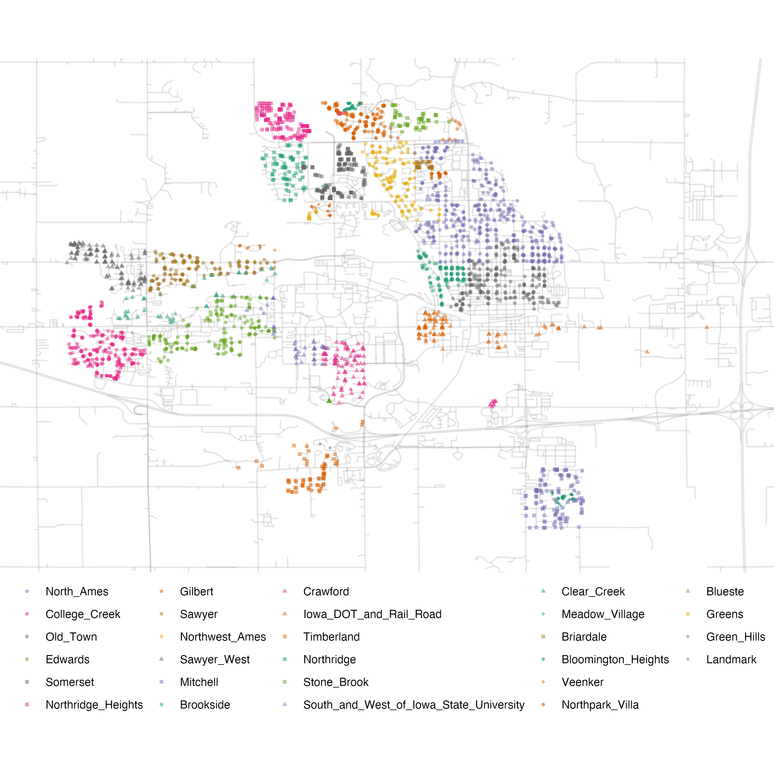
图 86.1: 这是数据故事的地图
这是一份Ames房屋数据,您可以把它想象为房屋中介推出的成都市武侯区、锦江区以及高新区等各区县的房屋信息
library(tidyverse)
ames <- read_csv("./demo_data/ames_houseprice.csv") %>%
        janitor::clean_names()

glimpse(ames)
## Rows: 1,460
## Columns: 81
## $ id <dbl> 1, 2, 3, 4, 5, 6, 7, 8, 9, 10, 11, 12, 13, 14, 15, 16,…
## $ ms_sub_class <dbl> 60, 20, 60, 70, 60, 50, 20, 60, 50, 190, 20, 60, 20, 2…
## $ ms_zoning <chr> "RL", "RL", "RL", "RL", "RL", "RL", "RL", "RL", "RM", …
## $ lot_frontage <dbl> 65, 80, 68, 60, 84, 85, 75, NA, 51, 50, 70, 85, NA, 91…
## $ lot_area <dbl> 8450, 9600, 11250, 9550, 14260, 14115, 10084, 10382, 6…
## $ street <chr> "Pave", "Pave", "Pave", "Pave", "Pave", "Pave", "Pave"…
## $ alley <chr> NA, NA, NA, NA, NA, NA, NA, NA, NA, NA, NA, NA, NA, NA…
## $ lot_shape <chr> "Reg", "Reg", "IR1", "IR1", "IR1", "IR1", "Reg", "IR1"…
## $ land_contour <chr> "Lvl", "Lvl", "Lvl", "Lvl", "Lvl", "Lvl", "Lvl", "Lvl"…
## $ utilities <chr> "AllPub", "AllPub", "AllPub", "AllPub", "AllPub", "All…
## $ lot_config <chr> "Inside", "FR2", "Inside", "Corner", "FR2", "Inside", …
## $ land_slope <chr> "Gtl", "Gtl", "Gtl", "Gtl", "Gtl", "Gtl", "Gtl", "Gtl"…
## $ neighborhood <chr> "CollgCr", "Veenker", "CollgCr", "Crawfor", "NoRidge",…
## $ condition1 <chr> "Norm", "Feedr", "Norm", "Norm", "Norm", "Norm", "Norm…
## $ condition2 <chr> "Norm", "Norm", "Norm", "Norm", "Norm", "Norm", "Norm"…
## $ bldg_type <chr> "1Fam", "1Fam", "1Fam", "1Fam", "1Fam", "1Fam", "1Fam"…
## $ house_style <chr> "2Story", "1Story", "2Story", "2Story", "2Story", "1.5…
## $ overall_qual <dbl> 7, 6, 7, 7, 8, 5, 8, 7, 7, 5, 5, 9, 5, 7, 6, 7, 6, 4, …
## $ overall_cond <dbl> 5, 8, 5, 5, 5, 5, 5, 6, 5, 6, 5, 5, 6, 5, 5, 8, 7, 5, …
## $ year_built <dbl> 2003, 1976, 2001, 1915, 2000, 1993, 2004, 1973, 1931, …
## $ year_remod_add <dbl> 2003, 1976, 2002, 1970, 2000, 1995, 2005, 1973, 1950, …
## $ roof_style <chr> "Gable", "Gable", "Gable", "Gable", "Gable", "Gable", …
## $ roof_matl <chr> "CompShg", "CompShg", "CompShg", "CompShg", "CompShg",…
## $ exterior1st <chr> "VinylSd", "MetalSd", "VinylSd", "Wd Sdng", "VinylSd",…
## $ exterior2nd <chr> "VinylSd", "MetalSd", "VinylSd", "Wd Shng", "VinylSd",…
## $ mas_vnr_type <chr> "BrkFace", "None", "BrkFace", "None", "BrkFace", "None…
## $ mas_vnr_area <dbl> 196, 0, 162, 0, 350, 0, 186, 240, 0, 0, 0, 286, 0, 306…
## $ exter_qual <chr> "Gd", "TA", "Gd", "TA", "Gd", "TA", "Gd", "TA", "TA", …
## $ exter_cond <chr> "TA", "TA", "TA", "TA", "TA", "TA", "TA", "TA", "TA", …
## $ foundation <chr> "PConc", "CBlock", "PConc", "BrkTil", "PConc", "Wood",…
## $ bsmt_qual <chr> "Gd", "Gd", "Gd", "TA", "Gd", "Gd", "Ex", "Gd", "TA", …
## $ bsmt_cond <chr> "TA", "TA", "TA", "Gd", "TA", "TA", "TA", "TA", "TA", …
## $ bsmt_exposure <chr> "No", "Gd", "Mn", "No", "Av", "No", "Av", "Mn", "No", …
## $ bsmt_fin_type1 <chr> "GLQ", "ALQ", "GLQ", "ALQ", "GLQ", "GLQ", "GLQ", "ALQ"…
## $ bsmt_fin_sf1 <dbl> 706, 978, 486, 216, 655, 732, 1369, 859, 0, 851, 906, …
## $ bsmt_fin_type2 <chr> "Unf", "Unf", "Unf", "Unf", "Unf", "Unf", "Unf", "BLQ"…
## $ bsmt_fin_sf2 <dbl> 0, 0, 0, 0, 0, 0, 0, 32, 0, 0, 0, 0, 0, 0, 0, 0, 0, 0,…
## $ bsmt_unf_sf <dbl> 150, 284, 434, 540, 490, 64, 317, 216, 952, 140, 134, …
## $ total_bsmt_sf <dbl> 856, 1262, 920, 756, 1145, 796, 1686, 1107, 952, 991, …
## $ heating <chr> "GasA", "GasA", "GasA", "GasA", "GasA", "GasA", "GasA"…
## $ heating_qc <chr> "Ex", "Ex", "Ex", "Gd", "Ex", "Ex", "Ex", "Ex", "Gd", …
## $ central_air <chr> "Y", "Y", "Y", "Y", "Y", "Y", "Y", "Y", "Y", "Y", "Y",…
## $ electrical <chr> "SBrkr", "SBrkr", "SBrkr", "SBrkr", "SBrkr", "SBrkr", …
## $ x1st_flr_sf <dbl> 856, 1262, 920, 961, 1145, 796, 1694, 1107, 1022, 1077…
## $ x2nd_flr_sf <dbl> 854, 0, 866, 756, 1053, 566, 0, 983, 752, 0, 0, 1142, …
## $ low_qual_fin_sf <dbl> 0, 0, 0, 0, 0, 0, 0, 0, 0, 0, 0, 0, 0, 0, 0, 0, 0, 0, …
## $ gr_liv_area <dbl> 1710, 1262, 1786, 1717, 2198, 1362, 1694, 2090, 1774, …
## $ bsmt_full_bath <dbl> 1, 0, 1, 1, 1, 1, 1, 1, 0, 1, 1, 1, 1, 0, 1, 0, 1, 0, …
## $ bsmt_half_bath <dbl> 0, 1, 0, 0, 0, 0, 0, 0, 0, 0, 0, 0, 0, 0, 0, 0, 0, 0, …
## $ full_bath <dbl> 2, 2, 2, 1, 2, 1, 2, 2, 2, 1, 1, 3, 1, 2, 1, 1, 1, 2, …
## $ half_bath <dbl> 1, 0, 1, 0, 1, 1, 0, 1, 0, 0, 0, 0, 0, 0, 1, 0, 0, 0, …
## $ bedroom_abv_gr <dbl> 3, 3, 3, 3, 4, 1, 3, 3, 2, 2, 3, 4, 2, 3, 2, 2, 2, 2, …
## $ kitchen_abv_gr <dbl> 1, 1, 1, 1, 1, 1, 1, 1, 2, 2, 1, 1, 1, 1, 1, 1, 1, 2, …
## $ kitchen_qual <chr> "Gd", "TA", "Gd", "Gd", "Gd", "TA", "Gd", "TA", "TA", …
## $ tot_rms_abv_grd <dbl> 8, 6, 6, 7, 9, 5, 7, 7, 8, 5, 5, 11, 4, 7, 5, 5, 5, 6,…
## $ functional <chr> "Typ", "Typ", "Typ", "Typ", "Typ", "Typ", "Typ", "Typ"…
## $ fireplaces <dbl> 0, 1, 1, 1, 1, 0, 1, 2, 2, 2, 0, 2, 0, 1, 1, 0, 1, 0, …
## $ fireplace_qu <chr> NA, "TA", "TA", "Gd", "TA", NA, "Gd", "TA", "TA", "TA"…
## $ garage_type <chr> "Attchd", "Attchd", "Attchd", "Detchd", "Attchd", "Att…
## $ garage_yr_blt <dbl> 2003, 1976, 2001, 1998, 2000, 1993, 2004, 1973, 1931, …
## $ garage_finish <chr> "RFn", "RFn", "RFn", "Unf", "RFn", "Unf", "RFn", "RFn"…
## $ garage_cars <dbl> 2, 2, 2, 3, 3, 2, 2, 2, 2, 1, 1, 3, 1, 3, 1, 2, 2, 2, …
## $ garage_area <dbl> 548, 460, 608, 642, 836, 480, 636, 484, 468, 205, 384,…
## $ garage_qual <chr> "TA", "TA", "TA", "TA", "TA", "TA", "TA", "TA", "Fa", …
## $ garage_cond <chr> "TA", "TA", "TA", "TA", "TA", "TA", "TA", "TA", "TA", …
## $ paved_drive <chr> "Y", "Y", "Y", "Y", "Y", "Y", "Y", "Y", "Y", "Y", "Y",…
## $ wood_deck_sf <dbl> 0, 298, 0, 0, 192, 40, 255, 235, 90, 0, 0, 147, 140, 1…
## $ open_porch_sf <dbl> 61, 0, 42, 35, 84, 30, 57, 204, 0, 4, 0, 21, 0, 33, 21…
## $ enclosed_porch <dbl> 0, 0, 0, 272, 0, 0, 0, 228, 205, 0, 0, 0, 0, 0, 176, 0…
## $ x3ssn_porch <dbl> 0, 0, 0, 0, 0, 320, 0, 0, 0, 0, 0, 0, 0, 0, 0, 0, 0, 0…
## $ screen_porch <dbl> 0, 0, 0, 0, 0, 0, 0, 0, 0, 0, 0, 0, 176, 0, 0, 0, 0, 0…
## $ pool_area <dbl> 0, 0, 0, 0, 0, 0, 0, 0, 0, 0, 0, 0, 0, 0, 0, 0, 0, 0, …
## $ pool_qc <chr> NA, NA, NA, NA, NA, NA, NA, NA, NA, NA, NA, NA, NA, NA…
## $ fence <chr> NA, NA, NA, NA, NA, "MnPrv", NA, NA, NA, NA, NA, NA, N…
## $ misc_feature <chr> NA, NA, NA, NA, NA, "Shed", NA, "Shed", NA, NA, NA, NA…
## $ misc_val <dbl> 0, 0, 0, 0, 0, 700, 0, 350, 0, 0, 0, 0, 0, 0, 0, 0, 70…
## $ mo_sold <dbl> 2, 5, 9, 2, 12, 10, 8, 11, 4, 1, 2, 7, 9, 8, 5, 7, 3, …
## $ yr_sold <dbl> 2008, 2007, 2008, 2006, 2008, 2009, 2007, 2009, 2008, …
## $ sale_type <chr> "WD", "WD", "WD", "WD", "WD", "WD", "WD", "WD", "WD", …
## $ sale_condition <chr> "Normal", "Normal", "Normal", "Abnorml", "Normal", "No…
## $ sale_price <dbl> 208500, 181500, 223500, 140000, 250000, 143000, 307000…感谢曾倬同学提供的解释说明文档
explanation <- readxl::read_excel("./demo_data/ames_houseprice_explanation.xlsx")
explanation %>%
knitr::kable()| 列名 | description | 解释 |
|---|---|---|
| MSSubClass | Identifies the type of dwelling involved in the sale. | 住宅概况 |
| MSZoning | Identifies the general zoning classification of the sale. | 建筑性质(农业、商业、高/低密度住宅) |
| LotFrontage | Linear feet of street connected to property | 建筑离街道的距离 |
| LotArea | Lot size in square feet | 占地面积 |
| Street | Type of road access to property | 建筑附近的路面材质 |
| Alley | Type of alley access to property | 建筑附近小巷的修建材质 |
| LotShape | General shape of property | 建筑物的形状 |
| LandContour | Flatness of the property | 地面平坦程度 |
| Utilities | Type of utilities available | 可用公用设施类型 |
| LotConfig | Lot configuration | 房屋哪里配置多 |
| LandSlope | Slope of property | 建筑的斜率 |
| Neighborhood | Physical locations within Ames city limits | 建筑在Ames城市的位置 |
| Condition1 | Proximity to various conditions | 建筑附近的交通网络 |
| Condition2 | Proximity to various conditions (if more than one is present) | 建筑附近的交通网络 |
| BldgType | Type of dwelling | 住宅类别(联排别墅、独栋别墅…) |
| HouseStyle | Style of dwelling | 建筑风格 |
| OverallQual | Rates the overall material and finish of the house | 房屋装饰材质水平 |
| OverallCond | Rates the overall condition of the house | 房屋整体状况评估 |
| YearBuilt | Original construction date | 房屋修建日期 |
| YearRemodAdd | Remodel date (same as construction date if no remodeling or additions) | 房屋改建日期 |
| RoofStyle | Type of roof | 屋顶类型 |
| RoofMatl | Roof material | 屋顶材质 |
| Exterior1st | Exterior covering on house | 建筑外立面材质 |
| Exterior2nd | Exterior covering on house (if more than one material) | 建筑外立面材质 |
| MasVnrType | Masonry veneer type | 建筑表层砌体类型 |
| MasVnrArea | Masonry veneer area in square feet | 每平方英尺的砌体面积 |
| ExterQual | Evaluates the quality of the material on the exterior | 建筑表层砌体材料质量评估 |
| ExterCond | Evaluates the present condition of the material on the exterior | 建筑表层砌体材料现状评估 |
| Foundation | Type of foundation | 建筑基础的类型 |
| BsmtQual | Evaluates the height of the basement | 地下室高度评估 |
| BsmtCond | Evaluates the general condition of the basement | 地下室总体状况评估 |
| BsmtExposure | Refers to walkout or garden level walls | 走廊/花园外墙的评估 |
| BsmtFinType1 | Rating of basement finished area | 地下室完工区域的等级评价 |
| BsmtFinSF1 | Type 1 finished square feet | 地下室完工区域的面积 |
| BsmtFinType2 | Rating of basement finished area (if multiple types) | 其他地下室完工区域的等级评价 |
| BsmtFinSF2 | Type 2 finished square feet | 其他地下室完工区域的面积 |
| BsmtUnfSF | Unfinished square feet of basement area | 地下室未完工部分的面积 |
| TotalBsmtSF | Total square feet of basement area | 地下室总面积 |
| Heating | Type of heating | 房屋暖气类型(地暖、墙暖….) |
| HeatingQC | Heating quality and condition | 暖气设施的质量和条件 |
| CentralAir | Central air conditioning | 是否有中央空调 |
| Electrical | Electrical system | 电器系统配置标准 |
| 1stFlrSF | First Floor square feet | 一楼面积 |
| 2ndFlrSF | Second floor square feet | 二楼面积 |
| LowQualFinSF | Low quality finished square feet (all floors) | 所有楼层中低质量施工面积 |
| GrLivArea | Above grade (ground) living area square feet | 地上居住面积 |
| BsmtFullBath | Basement full bathrooms | 地下室标准卫生间个数 |
| BsmtHalfBath | Basement half bathrooms | 地下室简易卫生间个数 |
| FullBath | Full bathrooms above grade | 地上楼层标准卫生间个数 |
| HalfBath | Half baths above grade | 地上楼层简易卫生间个数 |
| BedroomAbvGr | Bedrooms above grade (does NOT include basement bedrooms) | 地上楼层卧室个数 |
| KitchenAbvGr | Kitchens above grade | 地上楼层厨房个数 |
| KitchenQual | Kitchen quality | 厨房质量评估 |
| TopRmsAbvGrd | Total rooms above grade (does not include bathrooms) | 地上楼层房间总数(除去卧室) |
| Functional | Home functionality (Assume typical unless deductions are warranted) | 房屋功能情况 |
| Fireplaces | Number of fireplaces | 壁炉个数 |
| FireplaceQu | Fireplace quality | 壁炉质量 |
| GarageType | Garage location | 车库位置 |
| GarageYrBlt | Year garage was built | 车库建成年份 |
| GarageFinish | Interior finish of the garage | 车库内部装饰情况 |
| GarageCars | Size of garage in car capacity | 车库容量 |
| GarageArea | Size of garage in square feet | 车库占地面积 |
| GarageQual | Garage quality | 车库质量 |
| GarageCond | Garage condition | 车库条件 |
| PavedDrive | Paved driveway | 车道施工方式 |
| WoodDeckSF | Wood deck area in square feet | 木甲板面积 |
| OpenPorchSF | Open porch area in square feet | 开放式门廊面积 |
| EnclosedPorch | Enclosed porch area in square feet | 封闭式门廊面积 |
| 3SsnPorch | Three season porch area in square feet | 三季门廊面积 |
| ScreenPorch | Screen porch area in square feet | 纱窗门廊面积 |
| PoolArea | Pool area in square feet | 游泳池面积 |
| PoolQC | Pool quality | 游泳池质量 |
| Fence | Fence quality | 栅栏质量 |
| MiscFeature | Miscellaneous feature not covered in other categories | 其他配套设施(网球场、电梯…) |
| MiscVal | $Value of miscellaneous feature | 其他配套设施的费用 |
| MoSold | Month Sold (MM) | 销售月份 |
| YrSold | Year Sold (YYYY) | 销售年份 |
| SaleType | Type of sale | 支付方式 |
| SaleCondition | Condition of sale | 房屋出售的情况 |
86.2 探索设想
- 读懂数据描述,比如
- 房屋设施 (bedrooms, garage, fireplace, pool, porch, etc.),
- 地理位置 (neighborhood),
- 土地信息 (zoning, shape, size, etc.),
- 品相等级
- 出售价格
- 探索影响房屋价格的因素
- 必要的预处理(缺失值处理、标准化、对数化等等)
- 必要的可视化(比如价格分布图等)
- 必要的统计(比如各地区房屋价格的均值)
- 合理选取若干预测变量,建立多元线性模型,并对模型结果给出解释
- 房屋价格与预测变量(房屋大小、在城市的位置、房屋类型、与街道的距离)
86.3 变量选取
我们选取下列变量:
- lot_frontage, 建筑离街道的距离
- lot_area, 占地面积
- neighborhood, 建筑在城市的位置
- gr_liv_area, 地上居住面积
- bldg_type, 住宅类别(联排别墅、独栋别墅…)
- year_built 房屋修建日期
d <- ames %>%
  select(sale_price,
         lot_frontage,
         lot_area,
         neighborhood,
         gr_liv_area,
         bldg_type,
         year_built
         )
d
## # A tibble: 1,460 × 7
## sale_price lot_frontage lot_area neighborhood gr_liv_area bldg_type
## <dbl> <dbl> <dbl> <chr> <dbl> <chr>
## 1 208500 65 8450 CollgCr 1710 1Fam
## 2 181500 80 9600 Veenker 1262 1Fam
## 3 223500 68 11250 CollgCr 1786 1Fam
## 4 140000 60 9550 Crawfor 1717 1Fam
## 5 250000 84 14260 NoRidge 2198 1Fam
## 6 143000 85 14115 Mitchel 1362 1Fam
## 7 307000 75 10084 Somerst 1694 1Fam
## 8 200000 NA 10382 NWAmes 2090 1Fam
## 9 129900 51 6120 OldTown 1774 1Fam
## 10 118000 50 7420 BrkSide 1077 2fmCon
## # ℹ 1,450 more rows
## # ℹ 1 more variable: year_built <dbl>86.4 缺失值处理
## # A tibble: 1 × 7
##   sale_price lot_frontage lot_area neighborhood gr_liv_area bldg_type year_built
##        <int>        <int>    <int>        <int>       <int>     <int>      <int>
## 1          0          259        0            0           0         0          0
找出来看看
d %>%
  filter_all(
    any_vars(is.na(.))
  )
## # A tibble: 259 × 7
## sale_price lot_frontage lot_area neighborhood gr_liv_area bldg_type
## <dbl> <dbl> <dbl> <chr> <dbl> <chr>
## 1 200000 NA 10382 NWAmes 2090 1Fam
## 2 144000 NA 12968 Sawyer 912 1Fam
## 3 157000 NA 10920 NAmes 1253 1Fam
## 4 149000 NA 11241 NAmes 1004 1Fam
## 5 154000 NA 8246 Sawyer 1060 1Fam
## 6 149350 NA 8544 Sawyer 1228 1Fam
## 7 144000 NA 9180 SawyerW 884 1Fam
## 8 130250 NA 9200 CollgCr 938 1Fam
## 9 177000 NA 13869 Gilbert 1470 1Fam
## 10 219500 NA 9375 CollgCr 2034 1Fam
## # ℹ 249 more rows
## # ℹ 1 more variable: year_built <dbl>如果不选择lot_frontage 就不会有缺失值,如何选择,自己抉择
我个人觉得这个变量很重要,所以还是保留,牺牲一点样本量吧
86.5 预处理
- 标准化
standard <- function(x) {
  (x - mean(x)) / sd(x)
}

d %>%
  mutate(
    across(where(is.numeric), standard),
    across(where(is.character), as.factor)
  )
## # A tibble: 1,201 × 7
## sale_price lot_frontage lot_area neighborhood gr_liv_area bldg_type
## <dbl> <dbl> <dbl> <fct> <dbl> <fct>
## 1 0.333 -0.208 -0.190 CollgCr 0.375 1Fam
## 2 0.00875 0.410 -0.0444 Veenker -0.470 1Fam
## 3 0.512 -0.0844 0.164 CollgCr 0.519 1Fam
## 4 -0.489 -0.414 -0.0507 Crawfor 0.388 1Fam
## 5 0.830 0.574 0.544 NoRidge 1.30 1Fam
## 6 -0.453 0.616 0.525 Mitchel -0.281 1Fam
## 7 1.51 0.204 0.0167 Somerst 0.345 1Fam
## 8 -0.610 -0.784 -0.484 OldTown 0.496 1Fam
## 9 -0.753 -0.826 -0.319 BrkSide -0.819 2fmCon
## 10 -0.615 -0.00206 0.158 Sawyer -0.889 1Fam
## # ℹ 1,191 more rows
## # ℹ 1 more variable: year_built <dbl>- 对数化
## # A tibble: 1,201 × 8
##    sale_price lot_frontage lot_area neighborhood gr_liv_area bldg_type
##         <dbl>        <dbl>    <dbl> <chr>              <dbl> <chr>
##  1     208500           65     8450 CollgCr             1710 1Fam
##  2     181500           80     9600 Veenker             1262 1Fam
##  3     223500           68    11250 CollgCr             1786 1Fam
##  4     140000           60     9550 Crawfor             1717 1Fam
##  5     250000           84    14260 NoRidge             2198 1Fam
##  6     143000           85    14115 Mitchel             1362 1Fam
##  7     307000           75    10084 Somerst             1694 1Fam
##  8     129900           51     6120 OldTown             1774 1Fam
##  9     118000           50     7420 BrkSide             1077 2fmCon
## 10     129500           70    11200 Sawyer              1040 1Fam
## # ℹ 1,191 more rows
## # ℹ 2 more variables: year_built <dbl>, log_sale_price <dbl>## # A tibble: 1,201 × 7
## sale_price lot_frontage lot_area neighborhood gr_liv_area bldg_type
## <dbl> <dbl> <dbl> <fct> <dbl> <fct>
## 1 12.2 4.17 9.04 CollgCr 7.44 1Fam
## 2 12.1 4.38 9.17 Veenker 7.14 1Fam
## 3 12.3 4.22 9.33 CollgCr 7.49 1Fam
## 4 11.8 4.09 9.16 Crawfor 7.45 1Fam
## 5 12.4 4.43 9.57 NoRidge 7.70 1Fam
## 6 11.9 4.44 9.55 Mitchel 7.22 1Fam
## 7 12.6 4.32 9.22 Somerst 7.43 1Fam
## 8 11.8 3.93 8.72 OldTown 7.48 1Fam
## 9 11.7 3.91 8.91 BrkSide 6.98 2fmCon
## 10 11.8 4.25 9.32 Sawyer 6.95 1Fam
## # ℹ 1,191 more rows
## # ℹ 1 more variable: year_built <dbl>- 标准化 vs 对数化
选择哪一种,我们看图说话
d %>%
  ggplot(aes(x = sale_price)) +
  geom_density()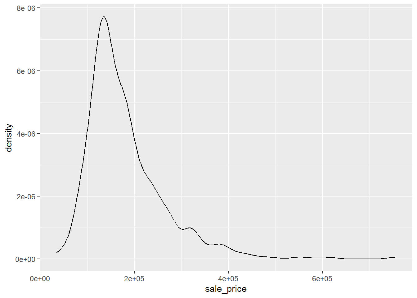
d %>%
  ggplot(aes(x = log(sale_price))) +
  geom_density()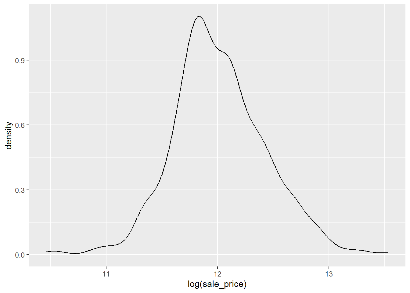
我们选择对数化,并保存结果
86.6 有趣的探索
86.6.1 各区域的房屋价格均值
## # A tibble: 25 × 2
##    neighborhood     n
##    <fct>        <int>
##  1 Blmngtn         14
##  2 Blueste          2
##  3 BrDale          16
##  4 BrkSide         51
##  5 ClearCr         13
##  6 CollgCr        126
##  7 Crawfor         41
##  8 Edwards         92
##  9 Gilbert         49
## 10 IDOTRR          34
## # ℹ 15 more rows
d %>%
group_by(neighborhood) %>%
summarise(
mean_sale = mean(sale_price)
) %>%
ggplot(
aes(x = mean_sale, y = fct_reorder(neighborhood, mean_sale))
) +
geom_col(aes(fill = mean_sale < 150000), show.legend = FALSE) +
geom_text(aes(label = round(mean_sale, 0)), hjust = 1) +
# scale_x_continuous(
# expand = c(0, 0),
# breaks = c(0, 100000, 200000, 300000),
# labels = c(0, "1w", "2w", "3w")
# ) +
scale_x_continuous(
expand = c(0, 0),
labels = scales::dollar
) +
scale_fill_viridis_d(option = "D") +
theme_classic() +
labs(x = NULL, y = NULL)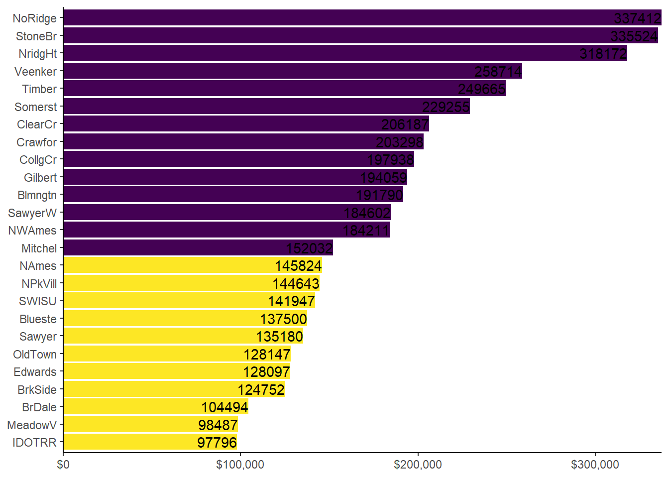
86.6.2 房屋价格与占地面积
d %>%
  ggplot(aes(x = log_lot_area, y = log_sale_price)) +
  geom_point(colour = "blue") +
  geom_smooth(method = lm, se = FALSE, formula = "y ~ x")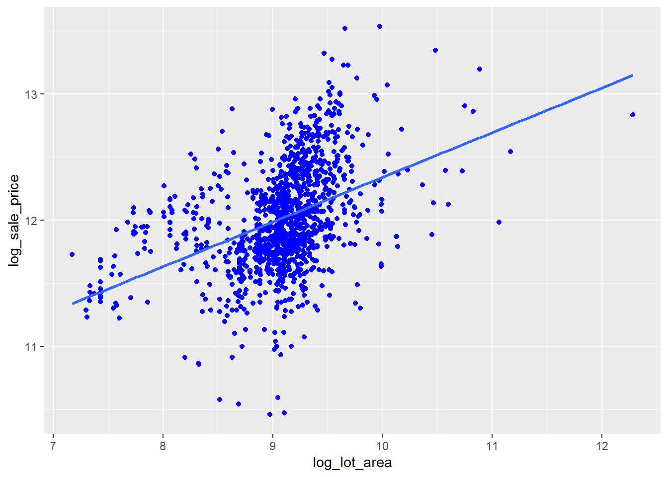
d %>%
  ggplot(aes(x = log_lot_area, y = log_sale_price)) +
  geom_point(aes(colour = neighborhood)) +
  geom_smooth(method = lm, se = FALSE, formula = "y ~ x")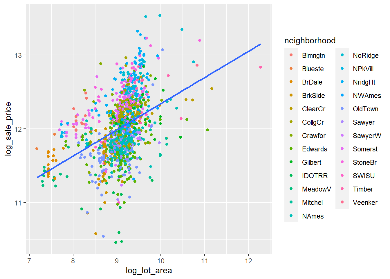
d %>%
  ggplot(aes(x = log_lot_area, y = log_sale_price)) +
  geom_point(colour = "blue") +
  geom_smooth(method = lm, se = FALSE, formula = "y ~ x", fullrange = TRUE) +
  facet_wrap(~neighborhood) +
  theme(strip.background = element_blank())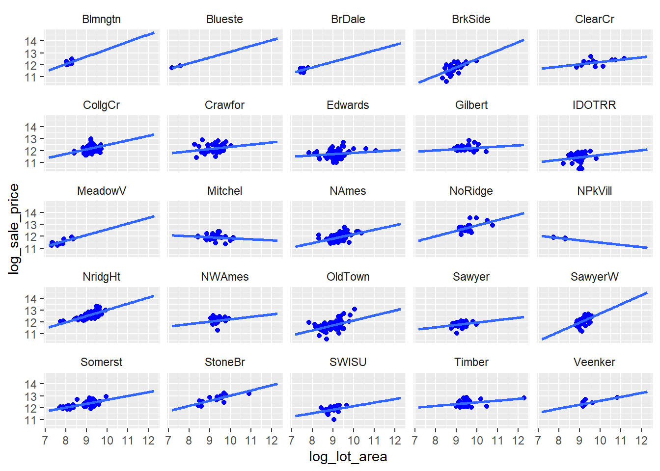
86.6.3 房屋价格与房屋居住面积
d %>%
  ggplot(aes(x = log_gr_liv_area, y = log_sale_price)) +
  geom_point(aes(colour = neighborhood)) +
  geom_smooth(method = lm, se = FALSE, formula = "y ~ x")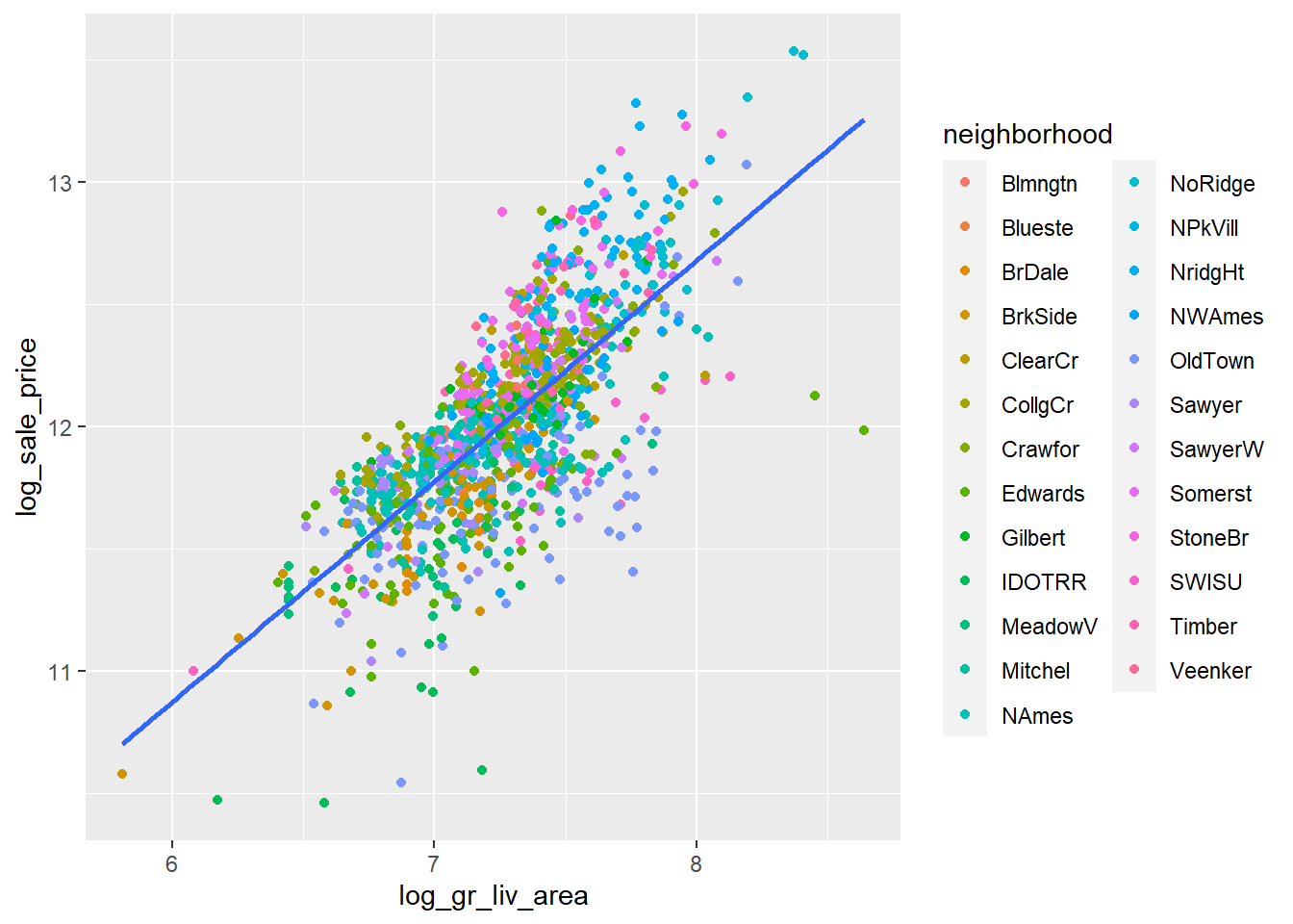
d %>%
  ggplot(aes(x = log_gr_liv_area, y = log_sale_price)) +
  geom_point() +
  geom_smooth(method = lm, se = FALSE, formula = "y ~ x", fullrange = TRUE) +
  facet_wrap(~neighborhood) +
  theme(strip.background = element_blank())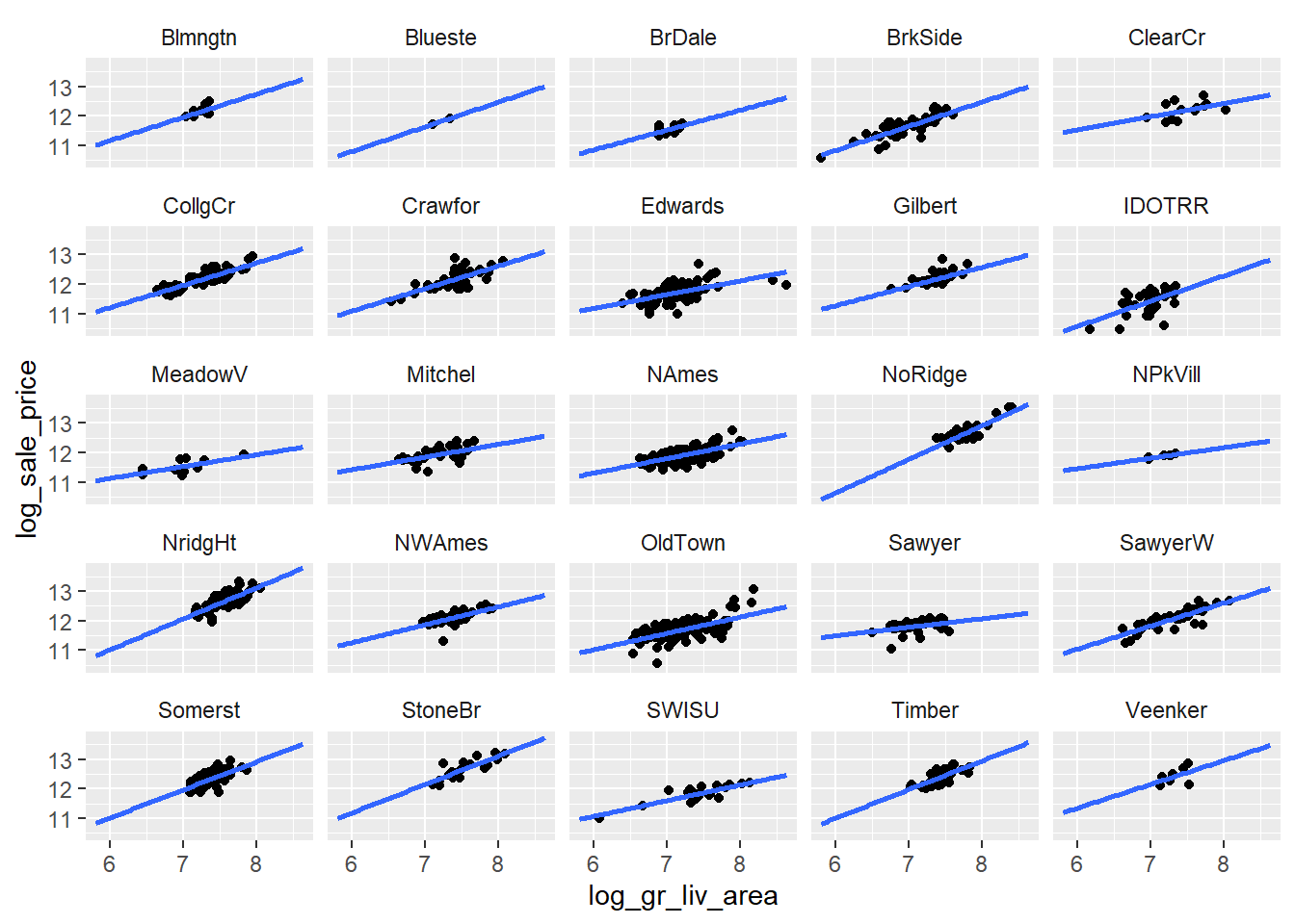
86.6.4 车库与房屋价格
车库大小是否对销售价格有帮助?
ames %>%
  #select(garage_cars, garage_area, sale_price) %>%
  ggplot(aes(x = garage_area, y = sale_price)) +
  geom_point(
    data = select(ames, -garage_cars),
    color = "gray50"
  ) +
  geom_point(aes(color = as_factor(garage_cars))) +
  facet_wrap(vars(garage_cars)) +
  theme(legend.position = "none") +
  ggtitle("This is the influence of garage for sale price")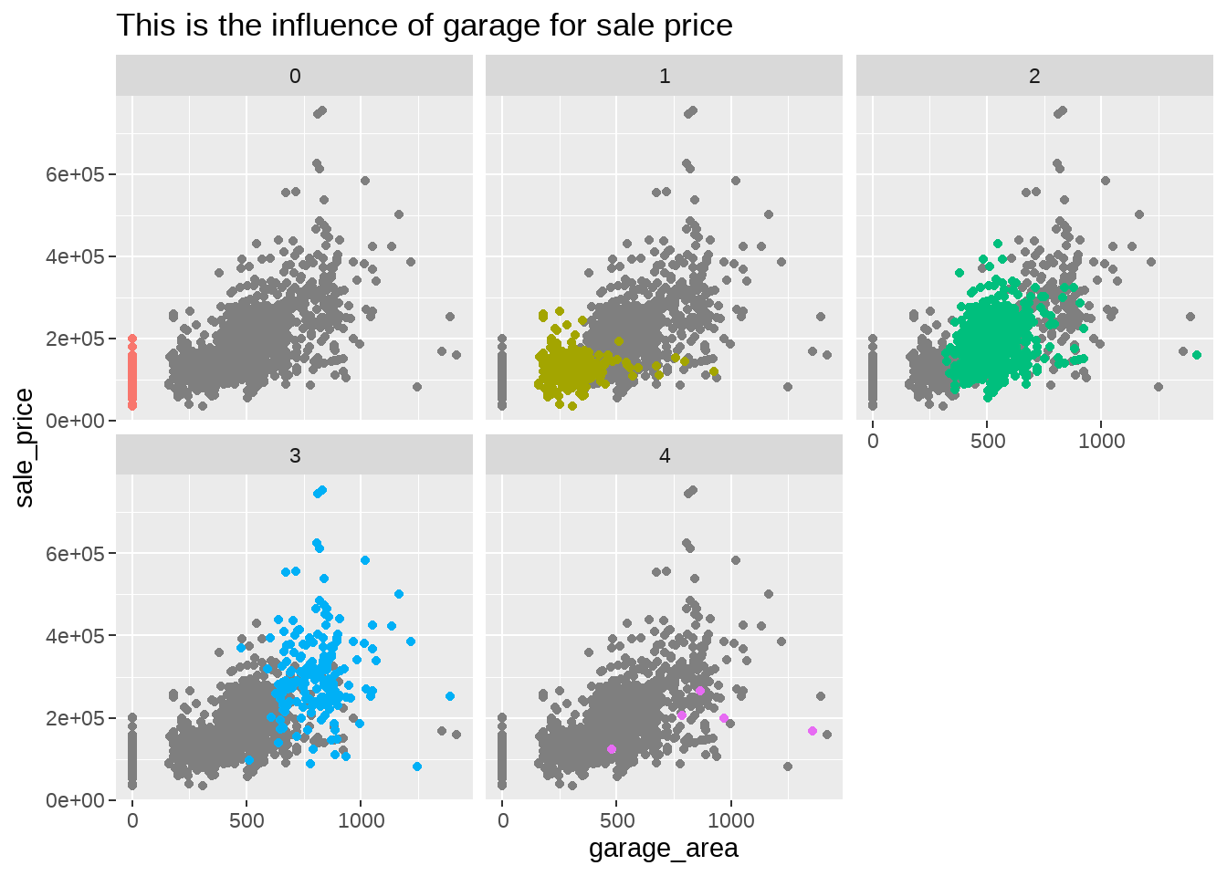
86.7 建模
## # A tibble: 26 × 5
##    term                estimate std.error statistic   p.value
##    <chr>                  <dbl>     <dbl>     <dbl>     <dbl>
##  1 (Intercept)          7.53       0.154    48.7    2.21e-284
##  2 log_gr_liv_area      0.638      0.0200   31.9    3.76e-161
##  3 neighborhoodBlueste -0.314      0.149    -2.10   3.55e-  2
##  4 neighborhoodBrDale  -0.466      0.0724   -6.43   1.80e- 10
##  5 neighborhoodBrkSide -0.336      0.0597   -5.62   2.44e-  8
##  6 neighborhoodClearCr -0.103      0.0762   -1.35   1.76e-  1
##  7 neighborhoodCollgCr  0.00332    0.0556    0.0597 9.52e-  1
##  8 neighborhoodCrawfor -0.0870     0.0612   -1.42   1.55e-  1
##  9 neighborhoodEdwards -0.365      0.0567   -6.44   1.79e- 10
## 10 neighborhoodGilbert -0.0621     0.0599   -1.04   3.00e-  1
## # ℹ 16 more rowslibrary(lme4)
lmer(log_sale_price ~ 1 + log_gr_liv_area + (log_gr_liv_area | neighborhood),
data = d) %>%
broom.mixed::tidy()## # A tibble: 6 × 6
## effect group term estimate std.error statistic
## <chr> <chr> <chr> <dbl> <dbl> <dbl>
## 1 fixed <NA> (Intercept) 6.88 0.334 20.6
## 2 fixed <NA> log_gr_liv_area 0.705 0.0493 14.3
## 3 ran_pars neighborhood sd__(Intercept) 1.34 NA NA
## 4 ran_pars neighborhood cor__(Intercept).log_gr_li… -0.993 NA NA
## 5 ran_pars neighborhood sd__log_gr_liv_area 0.205 NA NA
## 6 ran_pars Residual sd__Observation 0.191 NA NA