第 52 章 模型输出结果的规整
52.1 案例
还是用第 22 章的gapminder案例
## # A tibble: 1,704 × 6
##    country     continent  year lifeExp      pop gdpPercap
##    <fct>       <fct>     <int>   <dbl>    <int>     <dbl>
##  1 Afghanistan Asia       1952    28.8  8425333      779.
##  2 Afghanistan Asia       1957    30.3  9240934      821.
##  3 Afghanistan Asia       1962    32.0 10267083      853.
##  4 Afghanistan Asia       1967    34.0 11537966      836.
##  5 Afghanistan Asia       1972    36.1 13079460      740.
##  6 Afghanistan Asia       1977    38.4 14880372      786.
##  7 Afghanistan Asia       1982    39.9 12881816      978.
##  8 Afghanistan Asia       1987    40.8 13867957      852.
##  9 Afghanistan Asia       1992    41.7 16317921      649.
## 10 Afghanistan Asia       1997    41.8 22227415      635.
## # ℹ 1,694 more rows
52.1.1 可视化探索
画个简单的图
gapminder %>%
  ggplot(aes(x = log(gdpPercap), y = lifeExp)) +
  geom_point(alpha = 0.2)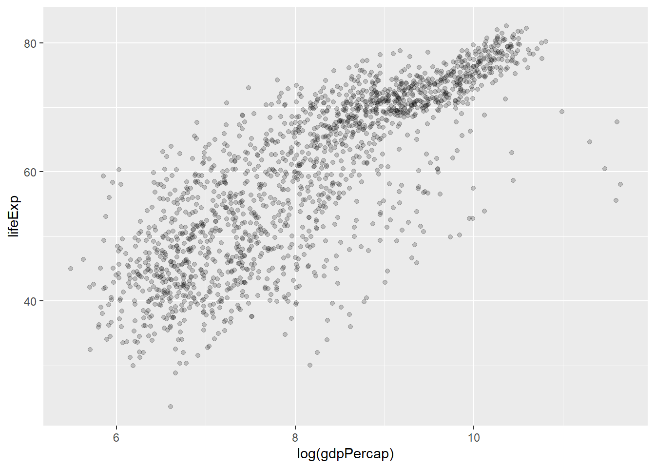
我们想用不同的模型拟合log(gdpPercap)与lifeExp的关联
library(colorspace)

model_colors <- colorspace::qualitative_hcl(4, palette = "dark 2")
# model_colors <- c("darkorange", "purple", "cyan4")

ggplot(
  data = gapminder,
  mapping = aes(x = log(gdpPercap), y = lifeExp)
) +
  geom_point(alpha = 0.2) +
  geom_smooth(
    method = "lm",
    aes(color = "OLS", fill = "OLS") # one
  ) +
  geom_smooth(
    method = "lm", formula = y ~ splines::bs(x, df = 3),
    aes(color = "Cubic Spline", fill = "Cubic Spline") # two
  ) +
  geom_smooth(
    method = "loess",
    aes(color = "LOESS", fill = "LOESS") # three
  ) +
  scale_color_manual(name = "Models", values = model_colors) +
  scale_fill_manual(name = "Models", values = model_colors) +
  theme(legend.position = "top")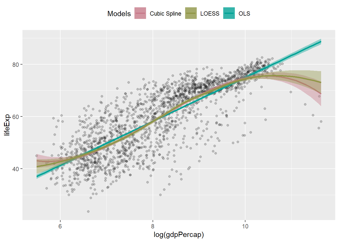
52.1.2 简单模型
还是回到我们今天的主题。我们建立一个简单的线性模型
out <- lm(
  formula = lifeExp ~ gdpPercap + pop + continent,
  data = gapminder
)
out
##
## Call:
## lm(formula = lifeExp ~ gdpPercap + pop + continent, data = gapminder)
##
## Coefficients:
## (Intercept) gdpPercap pop continentAmericas
## 4.781e+01 4.495e-04 6.570e-09 1.348e+01
## continentAsia continentEurope continentOceania
## 8.193e+00 1.747e+01 1.808e+01str(out)summary(out)##
## Call:
## lm(formula = lifeExp ~ gdpPercap + pop + continent, data = gapminder)
##
## Residuals:
## Min 1Q Median 3Q Max
## -49.161 -4.486 0.297 5.110 25.175
##
## Coefficients:
## Estimate Std. Error t value Pr(>|t|)
## (Intercept) 4.781e+01 3.395e-01 140.819 < 2e-16 ***
## gdpPercap 4.495e-04 2.346e-05 19.158 < 2e-16 ***
## pop 6.570e-09 1.975e-09 3.326 0.000901 ***
## continentAmericas 1.348e+01 6.000e-01 22.458 < 2e-16 ***
## continentAsia 8.193e+00 5.712e-01 14.342 < 2e-16 ***
## continentEurope 1.747e+01 6.246e-01 27.973 < 2e-16 ***
## continentOceania 1.808e+01 1.782e+00 10.146 < 2e-16 ***
## ---
## Signif. codes: 0 '***' 0.001 '**' 0.01 '*' 0.05 '.' 0.1 ' ' 1
##
## Residual standard error: 8.365 on 1697 degrees of freedom
## Multiple R-squared: 0.5821, Adjusted R-squared: 0.5806
## F-statistic: 393.9 on 6 and 1697 DF, p-value: < 2.2e-16out的结构

图 52.1: 线性模型结果的示意图
我们发现out对象包含了很多元素,比如系数、残差、模型残差自由度等等,用读取列表的方法可以直接读取
out$coefficients
out$residuals
out$fitted.values事实上,前面使用的suammary()函数只是选取和打印了out对象的一小部分信息,同时这些信息的结构不适合用dplyr操作和ggplot2画图。
52.2 broom
为规整模型结果,这里我们推荐用David Robinson 开发的broom宏包。
broom 宏包将常用的100多种模型的输出结果规整成数据框
tibble()的格式,在模型比较和可视化中就可以方便使用dplyr函数了。
broom 提供了三个主要的函数:
-
tidy()提取模型输出结果的主要信息,比如coefficients和t-statistics -
glance()把模型视为一个整体,提取如F-statistic,model deviance或者r-squared等信息 -
augment()模型输出的信息添加到建模用的数据集中,比如fitted values和residuals
52.2.1 tidy
tidy(out)## # A tibble: 7 × 5
## term estimate std.error statistic p.value
## <chr> <dbl> <dbl> <dbl> <dbl>
## 1 (Intercept) 4.78e+1 0.340 141. 0
## 2 gdpPercap 4.50e-4 0.0000235 19.2 3.24e- 74
## 3 pop 6.57e-9 0.00000000198 3.33 9.01e- 4
## 4 continentAmericas 1.35e+1 0.600 22.5 5.19e- 98
## 5 continentAsia 8.19e+0 0.571 14.3 4.06e- 44
## 6 continentEurope 1.75e+1 0.625 28.0 6.34e-142
## 7 continentOceania 1.81e+1 1.78 10.1 1.59e- 23out %>%
tidy() %>%
ggplot(mapping = aes(
x = term,
y = estimate
)) +
geom_point() +
coord_flip()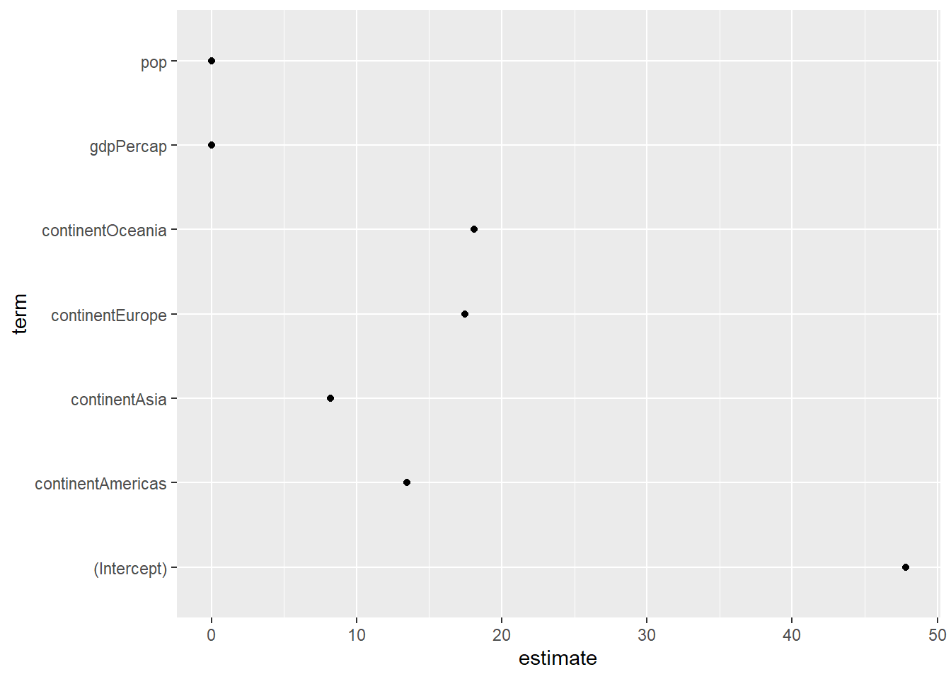
可以很方便的获取系数的置信区间
## # A tibble: 7 × 7
##   term              estimate    std.error statistic   p.value conf.low conf.high
##   <chr>                <dbl>        <dbl>     <dbl>     <dbl>    <dbl>     <dbl>
## 1 (Intercept)        4.78e+1      3.40e-1    141.   0          4.71e+1   4.85e+1
## 2 gdpPercap          4.50e-4      2.35e-5     19.2  3.24e- 74  4.03e-4   4.96e-4
## 3 pop                6.57e-9      1.98e-9      3.33 9.01e-  4  2.70e-9   1.04e-8
## 4 continentAmericas  1.35e+1      6.00e-1     22.5  5.19e- 98  1.23e+1   1.47e+1
## 5 continentAsia      8.19e+0      5.71e-1     14.3  4.06e- 44  7.07e+0   9.31e+0
## 6 continentEurope    1.75e+1      6.25e-1     28.0  6.34e-142  1.62e+1   1.87e+1
## 7 continentOceania   1.81e+1      1.78e+0     10.1  1.59e- 23  1.46e+1   2.16e+1
out %>%
tidy(conf.int = TRUE) %>%
filter(!term %in% c("(Intercept)")) %>%
ggplot(aes(
x = reorder(term, estimate),
y = estimate, ymin = conf.low, ymax = conf.high
)) +
geom_pointrange() +
coord_flip() +
labs(x = "", y = "OLS Estimate")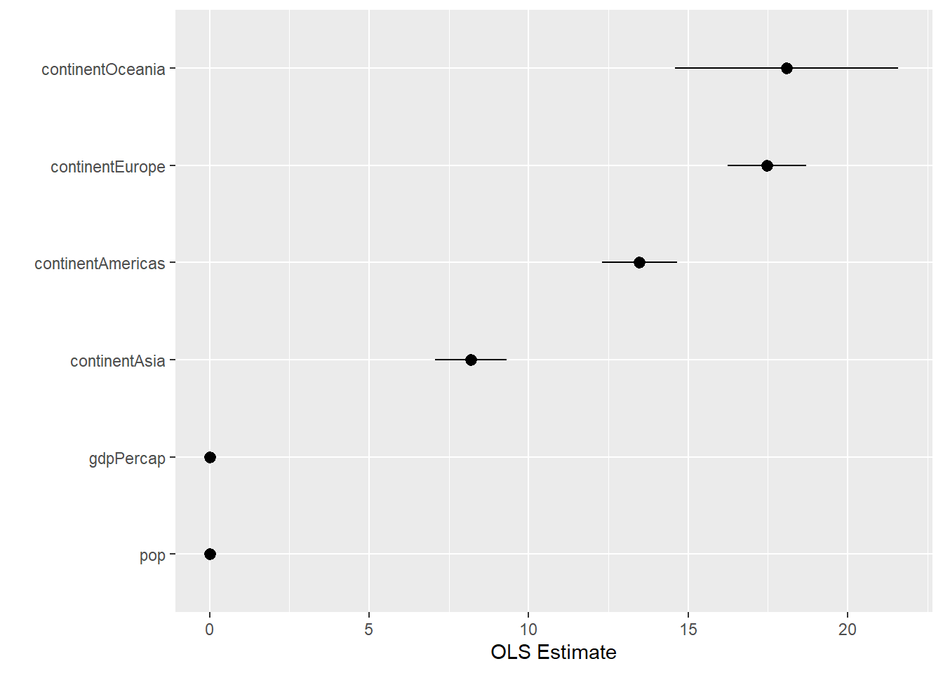
52.2.2 augment
augment()会返回一个数据框,这个数据框是在原始数据框的基础上,增加了模型的拟合值(.fitted), 拟合值的标准误(.se.fit), 残差(.resid)等列。
augment(out)## # A tibble: 1,704 × 10
## lifeExp gdpPercap pop continent .fitted .resid .hat .sigma .cooksd
## <dbl> <dbl> <int> <fct> <dbl> <dbl> <dbl> <dbl> <dbl>
## 1 28.8 779. 8425333 Asia 56.4 -27.6 0.00322 8.34 0.00505
## 2 30.3 821. 9240934 Asia 56.4 -26.1 0.00321 8.34 0.00450
## 3 32.0 853. 10267083 Asia 56.5 -24.5 0.00320 8.35 0.00393
## 4 34.0 836. 11537966 Asia 56.5 -22.4 0.00319 8.35 0.00330
## 5 36.1 740. 13079460 Asia 56.4 -20.3 0.00319 8.35 0.00271
## 6 38.4 786. 14880372 Asia 56.5 -18.0 0.00317 8.36 0.00212
## 7 39.9 978. 12881816 Asia 56.5 -16.7 0.00316 8.36 0.00181
## 8 40.8 852. 13867957 Asia 56.5 -15.7 0.00317 8.36 0.00160
## 9 41.7 649. 16317921 Asia 56.4 -14.7 0.00318 8.36 0.00142
## 10 41.8 635. 22227415 Asia 56.4 -14.7 0.00314 8.36 0.00139
## # ℹ 1,694 more rows
## # ℹ 1 more variable: .std.resid <dbl>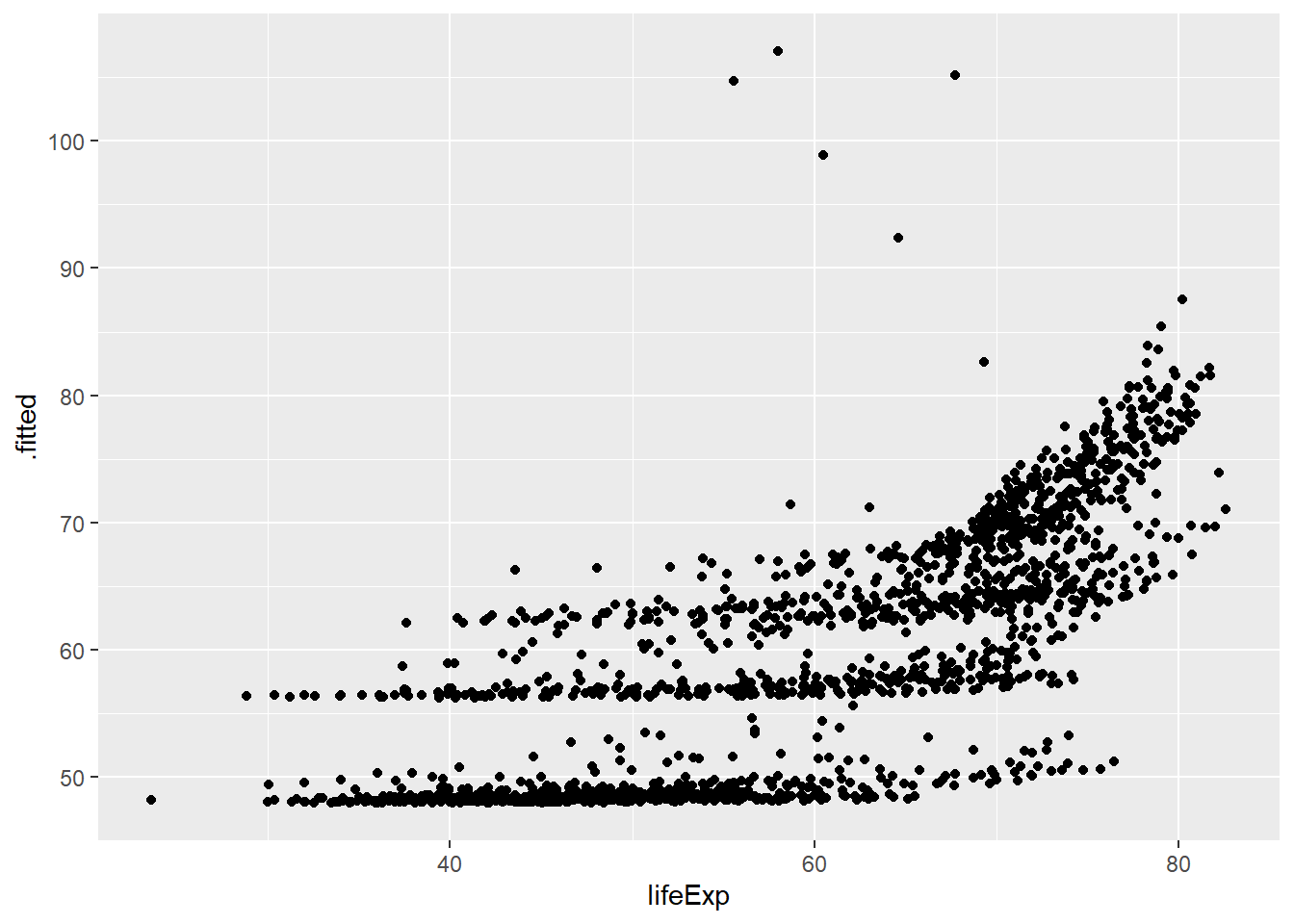
52.2.3 glance
glance() 函数也会返回数据框,但这个数据框只有一行,内容实际上是summary()输出结果的最底下一行。
glance(out)## # A tibble: 1 × 12
## r.squared adj.r.squared sigma statistic p.value df logLik AIC BIC
## <dbl> <dbl> <dbl> <dbl> <dbl> <dbl> <dbl> <dbl> <dbl>
## 1 0.582 0.581 8.37 394. 3.94e-317 6 -6034. 12084. 12127.
## # ℹ 3 more variables: deviance <dbl>, df.residual <int>, nobs <int>52.3 应用
broom的三个主要函数在分组统计建模时,格外方便。
penguins %>%
  group_nest(species) %>%
  mutate(model = purrr::map(data, ~ lm(bill_depth_mm ~ bill_length_mm, data = .))) %>%
  mutate(glance = purrr::map(model, ~ broom::glance(.))) %>%
  tidyr::unnest(glance)
## # A tibble: 3 × 15
## species data model r.squared adj.r.squared sigma statistic p.value df
## <fct> <list<ti> <lis> <dbl> <dbl> <dbl> <dbl> <dbl> <dbl>
## 1 Adelie [146 × 7] <lm> 0.149 0.143 1.13 25.2 1.51e- 6 1
## 2 Chinst… [68 × 7] <lm> 0.427 0.418 0.866 49.2 1.53e- 9 1
## 3 Gentoo [119 × 7] <lm> 0.428 0.423 0.749 87.5 7.34e-16 1
## # ℹ 6 more variables: logLik <dbl>, AIC <dbl>, BIC <dbl>, deviance <dbl>,
## # df.residual <int>, nobs <int>fit_ols <- function(df) {
lm(body_mass_g ~ bill_depth_mm + bill_length_mm, data = df)
}
out_tidy <- penguins %>%
group_nest(species) %>%
mutate(model = purrr::map(data, fit_ols)) %>%
mutate(tidy = purrr::map(model, ~ broom::tidy(.))) %>%
tidyr::unnest(tidy) %>%
dplyr::filter(!term %in% "(Intercept)")
out_tidy## # A tibble: 6 × 8
## species data model term estimate std.error statistic p.value
## <fct> <list<tibble[,7]>> <list> <chr> <dbl> <dbl> <dbl> <dbl>
## 1 Adelie [146 × 7] <lm> bill… 164. 25.1 6.51 1.17e-9
## 2 Adelie [146 × 7] <lm> bill… 64.8 11.5 5.64 8.88e-8
## 3 Chinstrap [68 × 7] <lm> bill… 159. 43.3 3.67 4.98e-4
## 4 Chinstrap [68 × 7] <lm> bill… 23.8 14.7 1.62 1.11e-1
## 5 Gentoo [119 × 7] <lm> bill… 255. 40.0 6.37 4.01e-9
## 6 Gentoo [119 × 7] <lm> bill… 54.7 12.7 4.30 3.54e-5out_tidy %>%
ggplot(aes(
x = species, y = estimate,
ymin = estimate - 2 * std.error,
ymax = estimate + 2 * std.error,
color = term
)) +
geom_pointrange(position = position_dodge(width = 0.25)) +
theme(legend.position = "top") +
labs(x = NULL, y = "Estimate", color = "coef")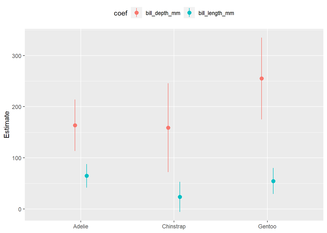
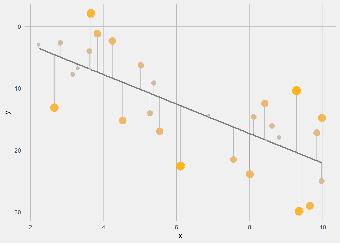
52.4 练习
假定数据是
## # A tibble: 30 × 2
##        x       y
##    <dbl>   <dbl>
##  1  5.55  -8.14
##  2  7.61 -15.2
##  3  4.13 -13.1
##  4  3.16  -9.92
##  5  6.50  -6.00
##  6  9.26 -25.7
##  7  6.22 -14.3
##  8  2.23   0.370
##  9  3.65 -12.3
## 10  6.98  -4.47
## # ℹ 20 more rows用broom::augment()和ggplot2做出类似的残差图