第 90 章 社会网络分析
本章通过tidygraph宏包介绍社会网络分析。社会网络分析涉及的知识比较多,而tidygraph将网络结构规整地比较清晰,降低了学习难度,很适合入门学习。
90.1 图论基本知识
网络图有两个主要特征: nodes and edges,
nodes:
edges:
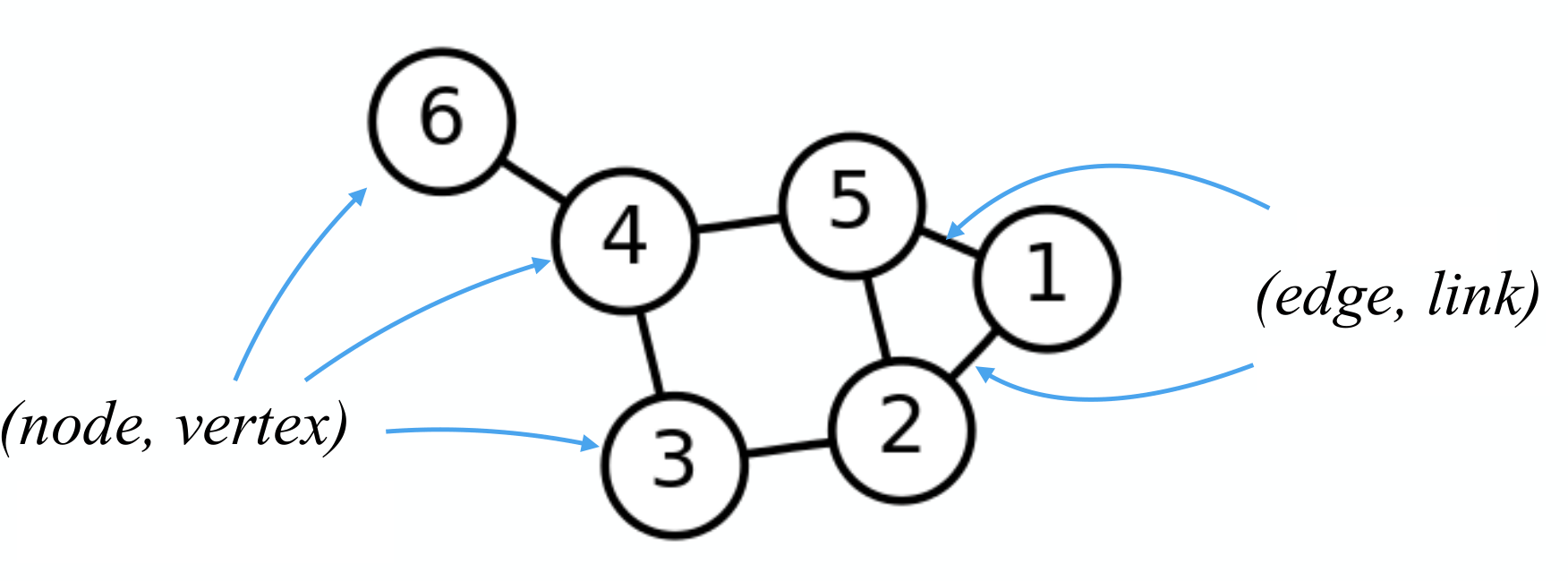
当然还包括其它的概念,比如
adjacency matrix:
edge list:
Node list:
Weighted network graph:
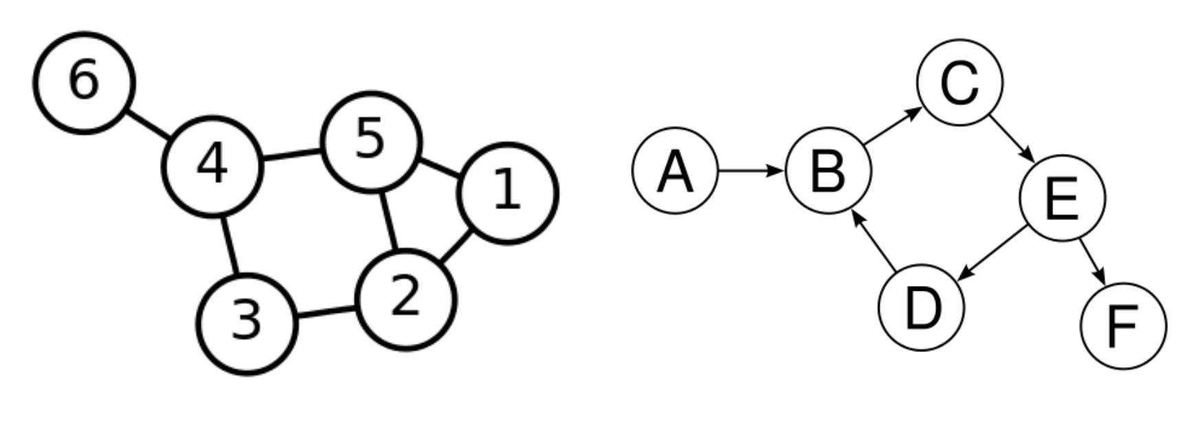
Directed and undirected network graph:
有向图
90.2 网络分析
先介绍tidygraph宏包
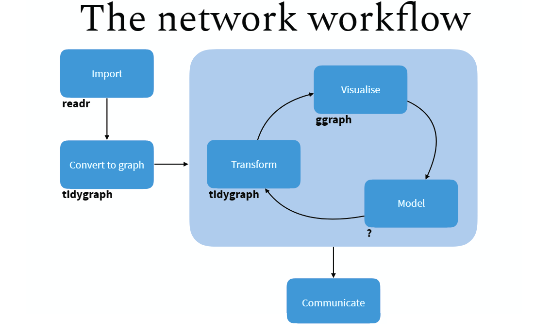
90.2.2 Tidy Network Anaylsis
- 在
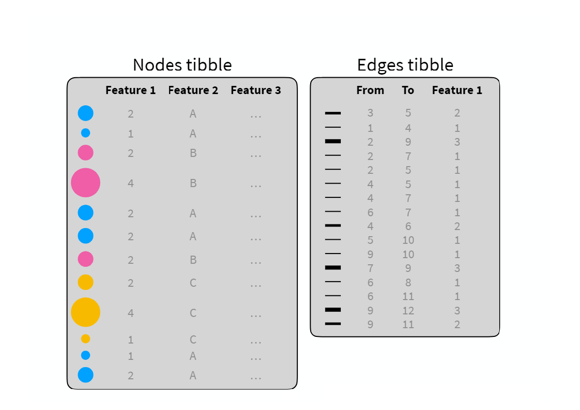
tidygraph框架, 网络数据可以分解成两个tidy数据框:- 一个是 node data
- 一个是 edge data
-
tidygraph宏包提供了node数据框和edge数据框相互切换的方案,并且可以使用dplyr的语法操控 -
tidygraph提供了常用的网络结构的algorithms,比如,计算网络拓扑结构中节点的重要性、中心度等。
90.2.3 Create network objects
创建网络对象主要有两个函数:
-
tbl_graph(). Creates a network object from nodes and edges data -
as_tbl_graph(). Converts network data and objects to atbl_graphnetwork.
案例: 欧盟总统之间通话以及次数。
node_list <- phone.call2$nodes
node_list
## # A tibble: 16 × 2
## id label
## <int> <chr>
## 1 1 France
## 2 2 Belgium
## 3 3 Germany
## 4 4 Danemark
## 5 5 Croatia
## 6 6 Slovenia
## 7 7 Hungary
## 8 8 Spain
## 9 9 Italy
## 10 10 Netherlands
## 11 11 UK
## 12 12 Austria
## 13 13 Poland
## 14 14 Switzerland
## 15 15 Czech republic
## 16 16 Slovaniaedge_list <- phone.call2$edges
edge_list## # A tibble: 18 × 3
## from to weight
## <int> <int> <dbl>
## 1 1 3 9
## 2 2 1 4
## 3 1 8 3
## 4 1 9 4
## 5 1 10 2
## 6 1 11 3
## 7 3 12 2
## 8 3 13 2
## 9 2 3 3
## 10 3 14 2
## 11 3 15 2
## 12 3 10 2
## 13 4 3 2
## 14 5 3 2
## 15 5 16 2
## 16 5 7 2
## 17 6 3 2
## 18 7 16 2.5
90.2.4 Use tbl_graph
- Create a
tbl_graphnetwork object using the phone call data:
phone.net <- tbl_graph(nodes = node_list, edges = edge_list, directed = TRUE)- Visualize the network graph
ggraph(phone.net, layout = "graphopt") +
  geom_edge_link(width = 1, colour = "lightgray") +
  geom_node_point(size = 4, colour = "red") +
  geom_node_text(aes(label = label), repel = TRUE) +
  theme_graph()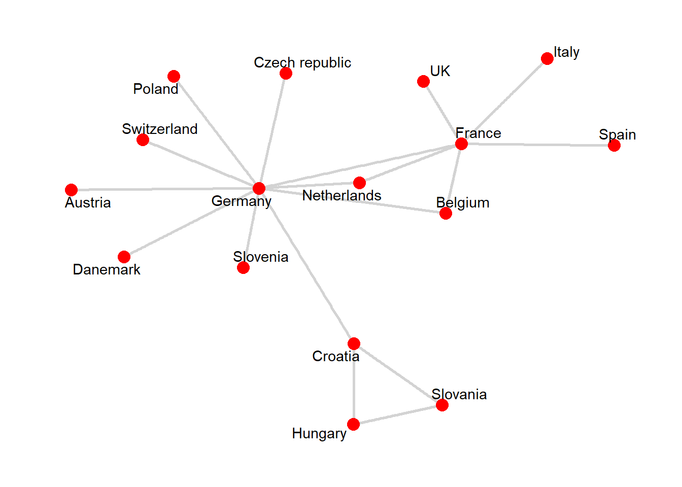
90.2.5 Use as_tbl_graph
mtcars data set: R 的内置数据集,记录了32种不同品牌的轿车的的11个属性
1、we create a correlation matrix network graph
library(corrr)
res.cor <- datasets::mtcars[, c(1, 3:6)] %>% # (1)
  t() %>%
  corrr::correlate() %>% # (2)
  corrr::shave(upper = TRUE) %>% # (3)
  corrr::stretch(na.rm = TRUE) %>% # (4)
  dplyr::filter(r >= 0.998) # (5)
res.cor
2、Create the correlation network graph:
set.seed(1)
cor.graph <- as_tbl_graph(res.cor, directed = FALSE)ggraph(cor.graph) +
geom_edge_link() +
geom_node_point() +
geom_node_text(
aes(label = name),
size = 3, repel = TRUE
) +
theme_graph()90.3 Network graph manipulation
90.3.5 Visualize the correlation network
set.seed(1)
ggraph(cor.graph) +
  geom_edge_link(aes(width = weight), alpha = 0.2) +
  scale_edge_width(range = c(0.2, 1)) +
  geom_node_point(aes(color = cyl), size = 2) +
  geom_node_text(aes(label = label), size = 3, repel = TRUE) +
  theme_graph()
90.4 Network analysis
90.4.1 Centrality
Centrality is an important concept when analyzing network graph.
The tidygraph package contains more than 10 centrality measures, prefixed with the term centrality_ :
# centrality_alpha()
# centrality_power()
# centrality_authority()
# centrality_betweenness()
# centrality_closeness()
# centrality_hub()
# centrality_degree()
# centrality_pagerank()
# centrality_eigen()
# centrality_subgraph
# centrality_edge_betweenness()
example: - use the phone call network graph ( 欧盟总统之间通话以及次数) - compute nodes centrality
set.seed(123)
phone.net %>%
  activate(nodes) %>%
mutate(centrality = centrality_authority()) %>%
ggraph(layout = "graphopt") +
geom_edge_link(width = 1, colour = "lightgray") +
geom_node_point(aes(size = centrality, colour = centrality)) +
geom_node_text(aes(label = label), repel = TRUE) +
scale_color_gradient(low = "yellow", high = "red") +
theme_graph()90.4.2 Clustering
Clustering is a common operation in network analysis and it consists of grouping nodes based on the graph topology.
-
Many clustering algorithms from are available in the tidygraph package and prefixed with the term group_. These include:
-
Infomap community finding. It groups nodes by minimizing the expected description length of a random walker trajectory. R function:
group_infomap() -
Community structure detection based on edge betweenness. It groups densely connected nodes. R function:
group_edge_betweenness()
-
Infomap community finding. It groups nodes by minimizing the expected description length of a random walker trajectory. R function:
example: - use the correlation network graphs (记录了32种不同品牌的轿车的的11个属性) - detect clusters or communities
set.seed(123)
cluster_mtcars <- cor.graph %>%
  activate(nodes) %>%
  mutate(community = as.factor(group_infomap()))
cluster_mtcars
cluster_mtcars %>%
ggraph(layout = "graphopt") +
geom_edge_link(width = 1, colour = "lightgray") +
geom_node_point(aes(colour = community), size = 4) +
geom_node_text(aes(label = label), repel = TRUE) +
theme_graph()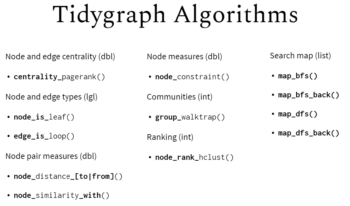
90.5 小结
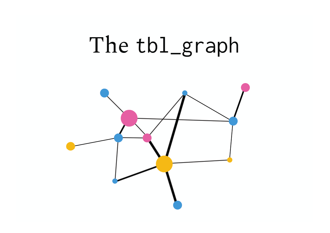
tidybayes很聪明地将复杂的网络结构用两个数据框表征出来,node 数据框负责节点的属性,edge 数据框负责网络连接的属性,调整其中的一个数据框,另一个也会相应的调整,比如node数据框中删除一个节点,edge数据框就会自动地删除该节点的所有连接。
90.6 Network Visualization
这里主要介绍tidygraph配套的ggraph宏包,它们的作者都是同一个人。
90.6.1 ggraph: A grammar of graphics for relational data
ggraph 沿袭了ggplot2的语法规则,
cluster_mtcars %>%
  # Layout
  ggraph(layout = "graphopt") +
  # Edges
  geom_edge_link(
    width = 1,
    colour = "lightgray"
  ) +
  # Nodes
  geom_node_point(
    aes(colour = community),
    size = 4
  ) +
  geom_node_text(
    aes(label = label),
    repel = TRUE
  ) +
  theme_graph()