第 32 章 ggplot2之科研数据可视化

## Warning: package 'ggplot2' was built under R version 4.2.3

## Warning: package 'tibble' was built under R version 4.2.3

## Warning: package 'tidyr' was built under R version 4.2.2

## Warning: package 'readr' was built under R version 4.2.2

## Warning: package 'purrr' was built under R version 4.2.2

## Warning: package 'dplyr' was built under R version 4.2.3

## Warning: package 'stringr' was built under R version 4.2.2

## Warning: package 'lubridate' was built under R version 4.2.2

## Warning: package 'ggridges' was built under R version 4.2.2

32.1 统计分布图

在学术中，很多情形我们都需要画出统计分布图。比如，围绕天气温度数据(美国内布拉斯加州东部，林肯市， 2016年)，我们想看每个月份里气温的分布情况

lincoln_df <- ggridges::lincoln_weather %>%
  mutate(
    month_short = fct_recode(
      Month,
      Jan = "January",
      Feb = "February",
      Mar = "March",
      Apr = "April",
      May = "May",
      Jun = "June",
      Jul = "July",
      Aug = "August",
      Sep = "September",
      Oct = "October",
      Nov = "November",
      Dec = "December"
    )
  ) %>%
  mutate(month_short = fct_rev(month_short)) %>%
  select(Month, month_short, `Mean Temperature [F]`)

lincoln_df %>%
  head(5)

## # A tibble: 5 × 3
##   Month   month_short `Mean Temperature [F]`
##   <fct>   <fct>                        <int>
## 1 January Jan                             24
## 2 January Jan                             23
## 3 January Jan                             23
## 4 January Jan                             17
## 5 January Jan                             29

统计分布图的方法很多，我们下面比较各种方法的优劣。

32.1.1 points-errorbars

画分布图的最简单的方法，就是计算每个月的气温均值或者中位数，并在均值或者中位数位置标出误差棒(error bars)，比如图 32.1 。

lincoln_errbar <- lincoln_df %>%
  ggplot(aes(x = month_short, y = `Mean Temperature [F]`)) +
  stat_summary(
    fun.y = mean, fun.ymax = function(x) {
      mean(x) + 2 * sd(x)
    },
    fun.ymin = function(x) {
      mean(x) - 2 * sd(x)
    }, geom = "pointrange",
    fatten = 5
  ) +
  xlab("month") +
  ylab("mean temperature (°F)") +
  theme_classic(base_size = 14) +
  theme(
    axis.text = element_text(color = "black", size = 12),
    plot.margin = margin(3, 7, 3, 1.5)
  )

## Warning: The `fun.y` argument of `stat_summary()` is deprecated as of ggplot2 3.3.0.
## ℹ Please use the `fun` argument instead.
## This warning is displayed once every 8 hours.
## Call `lifecycle::last_lifecycle_warnings()` to see where this warning was
## generated.

## Warning: The `fun.ymin` argument of `stat_summary()` is deprecated as of ggplot2 3.3.0.
## ℹ Please use the `fun.min` argument instead.
## This warning is displayed once every 8 hours.
## Call `lifecycle::last_lifecycle_warnings()` to see where this warning was
## generated.

## Warning: The `fun.ymax` argument of `stat_summary()` is deprecated as of ggplot2 3.3.0.
## ℹ Please use the `fun.max` argument instead.
## This warning is displayed once every 8 hours.
## Call `lifecycle::last_lifecycle_warnings()` to see where this warning was
## generated.

lincoln_errbar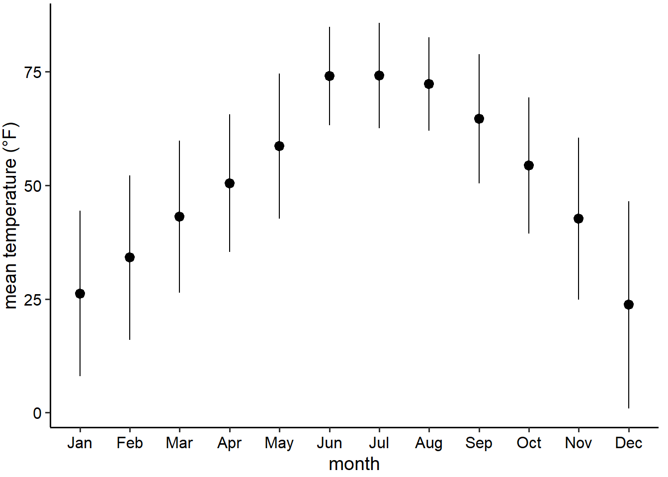

图 32.1: 林肯市2016年气温变化图

但这个图有很多问题，或者说是错误的

图中只用了一个点和两个误差棒，丢失了很多分布信息。
读者不能很直观的读出这个点的含义（是均值还是中位数？）
误差棒代表的含义不明确（标准差？标准误？还是其他？）

通过看代码，知道这里用的是，均值加减2倍的标准差，其目的是想表达这个范围涵盖了95%的的数据。事实上，误差棒一般用于标准误（或者加减2倍的标准误来代表估计均值的95%置信区间），所以这里使用标准差就造成了混淆。

( 标准误：对样本均值估计的不确定性; 标准差：对偏离均值的分散程度 )

现实的数据往往是偏态的，但这个图的误差棒几乎是对称，会让人觉得产生怀疑。

32.1.2 箱线图

为了解决以上问题，可以使用箱线图（boxplot），箱线图将数据分成若干段，如图 32.2.

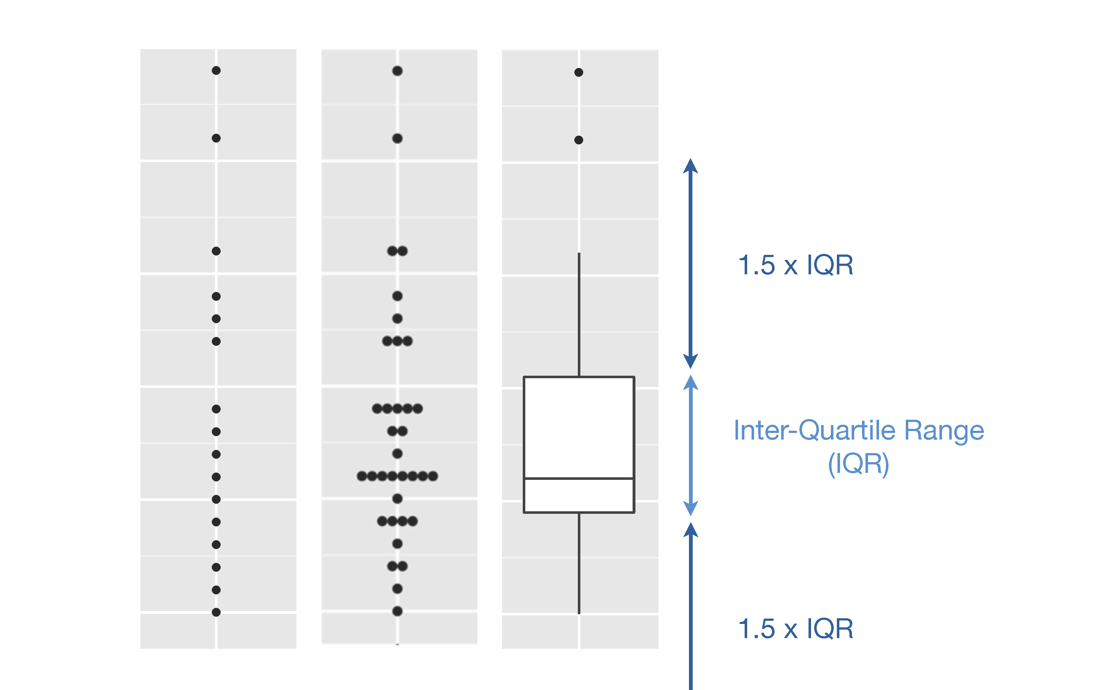
图 32.2: 箱线图示意图

盒子中间的横线是中位数(50th percentile)，底部的横线代表第一分位数(25th percentile)，顶部的横线代表第三分位数(75th percentile)
盒子的范围覆盖了50%的数据，每个小盒子是25%的数据，盒子高度越短，说明数据越集中，盒子高度越长，数据越分散。
上面的这条竖线的长度 = 从盒子上边缘开始，延伸到1.5倍盒子高度的范围中最远的点
下面的这条竖线的长度 = 从盒子下边缘开始，延伸到1.5倍盒子高度的范围中最远的点
在线条之外的点就是 outlies

那么气温分布用箱线图画出来 (图 32.3)。我们可以看到12月份数据偏态（绝大部分时候中等的冷，少部分是极度寒冷），其他月份，比如7月份，数据分布的比较正态

lincoln_box <- lincoln_df %>%
  ggplot(aes(x = month_short, y = `Mean Temperature [F]`)) +
  geom_boxplot(fill = "grey90") +
  xlab("month") +
  ylab("mean temperature (°F)") +
  theme_classic(base_size = 14) +
  theme(
    axis.text = element_text(color = "black", size = 12),
    plot.margin = margin(3, 7, 3, 1.5)
  )

lincoln_box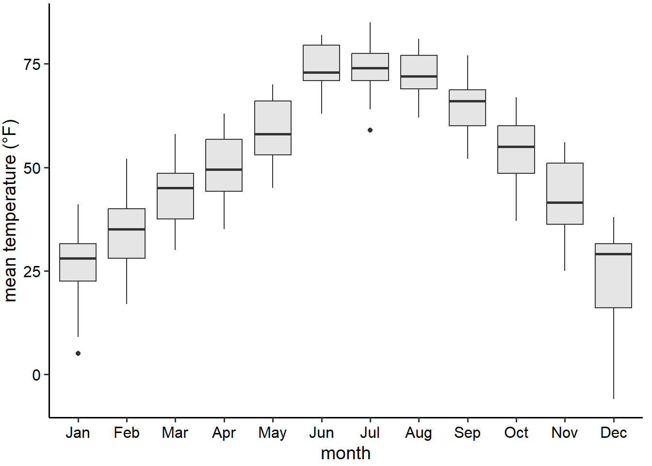

图 32.3: 林肯市2016年气温分布箱线图

32.1.3 小提琴图

箱线图是1970年代统计学家发明的一种可视化方法，这种图可以很方便地用手工画出，所以当时很流行，现在计算机性能大大提升了，所以大家喜欢用视觉上更直观的小提琴图取代箱线图

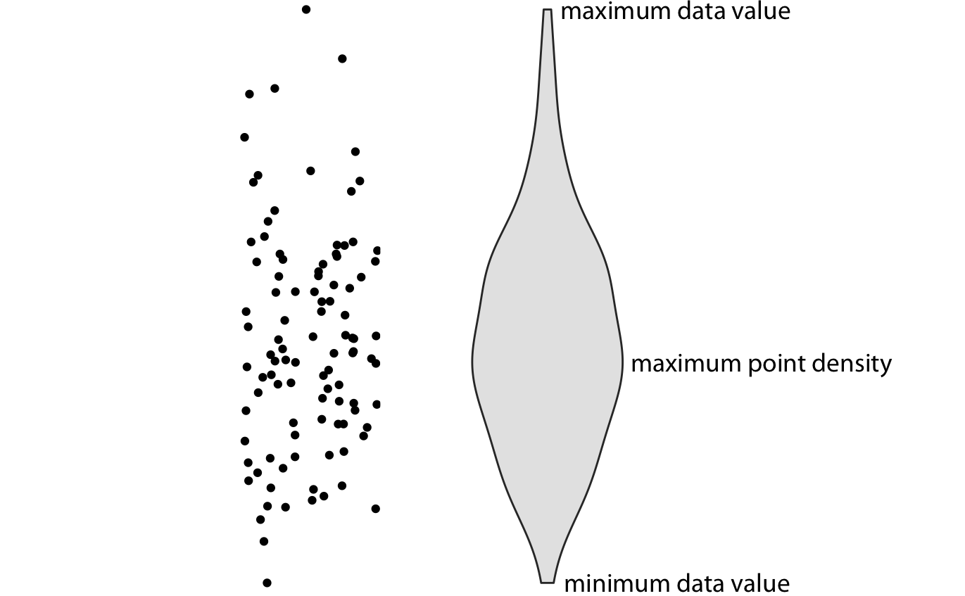
图 32.4: 小提琴图示意图

小提琴图相当于密度分布图旋转90度，然后再做个对称的镜像
最宽或者最厚的地方，对应着数据密度最大的地方
箱线图能用的地方小提琴图都能用，而且小提琴图可以很好的展示bimodal data的情况（箱线图做不到）

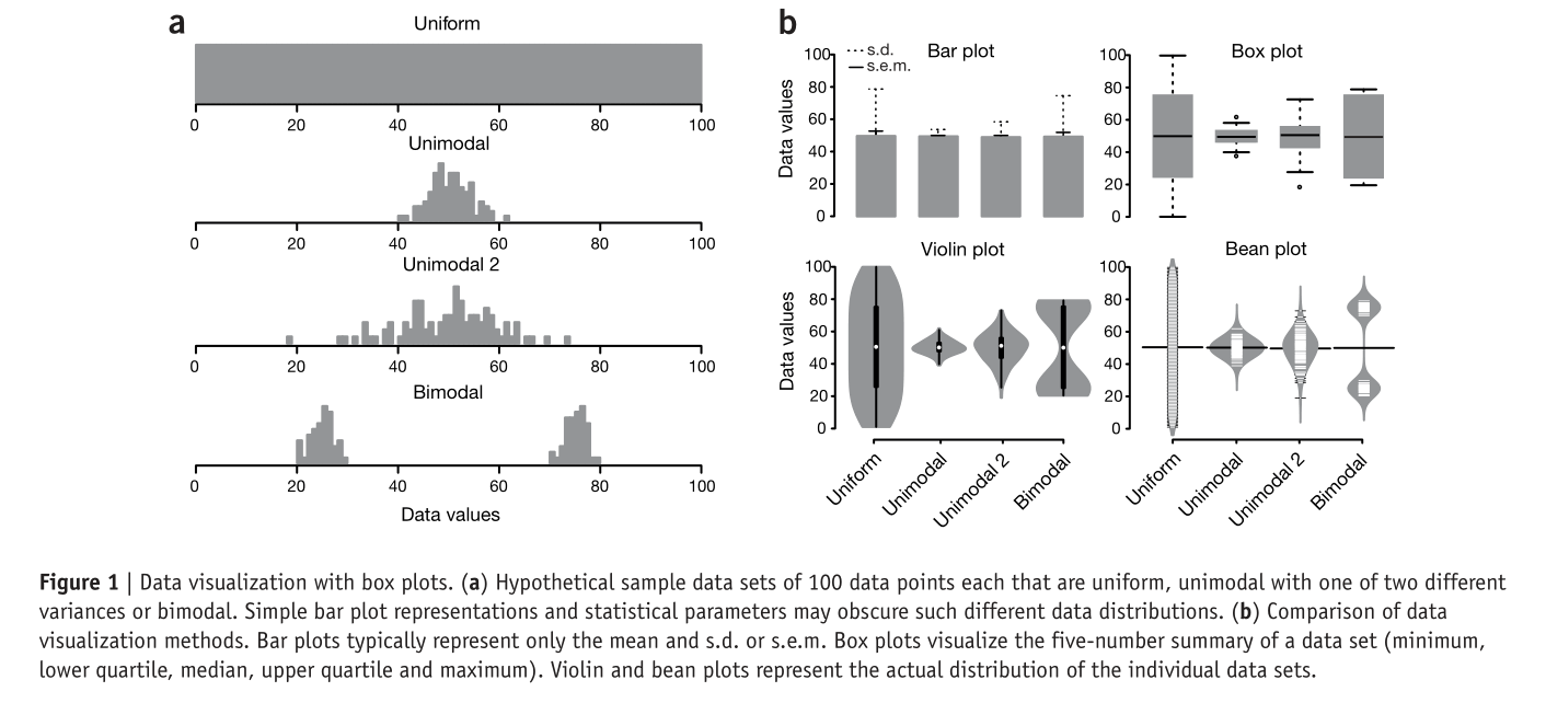
图 32.5: 图片来源：nature methods, VOL.11, NO.2, FEBRUARY 2014

在图 32.6，我们使用小提琴图画图气温分布，可以看到，11月份的时候，有两个高密度区间（两个峰，50 degrees 和 35 degrees Fahrenheit），注意，这个信息在前面两个图中是没有的。

lincoln_violin <- lincoln_df %>%
  ggplot(aes(x = month_short, y = `Mean Temperature [F]`)) +
  geom_violin(fill = "grey90") +
  xlab("month") +
  ylab("mean temperature (°F)") +
  theme_classic(base_size = 14) +
  theme(
    axis.text = element_text(color = "black", size = 12),
    plot.margin = margin(3, 7, 3, 1.5)
  )

lincoln_violin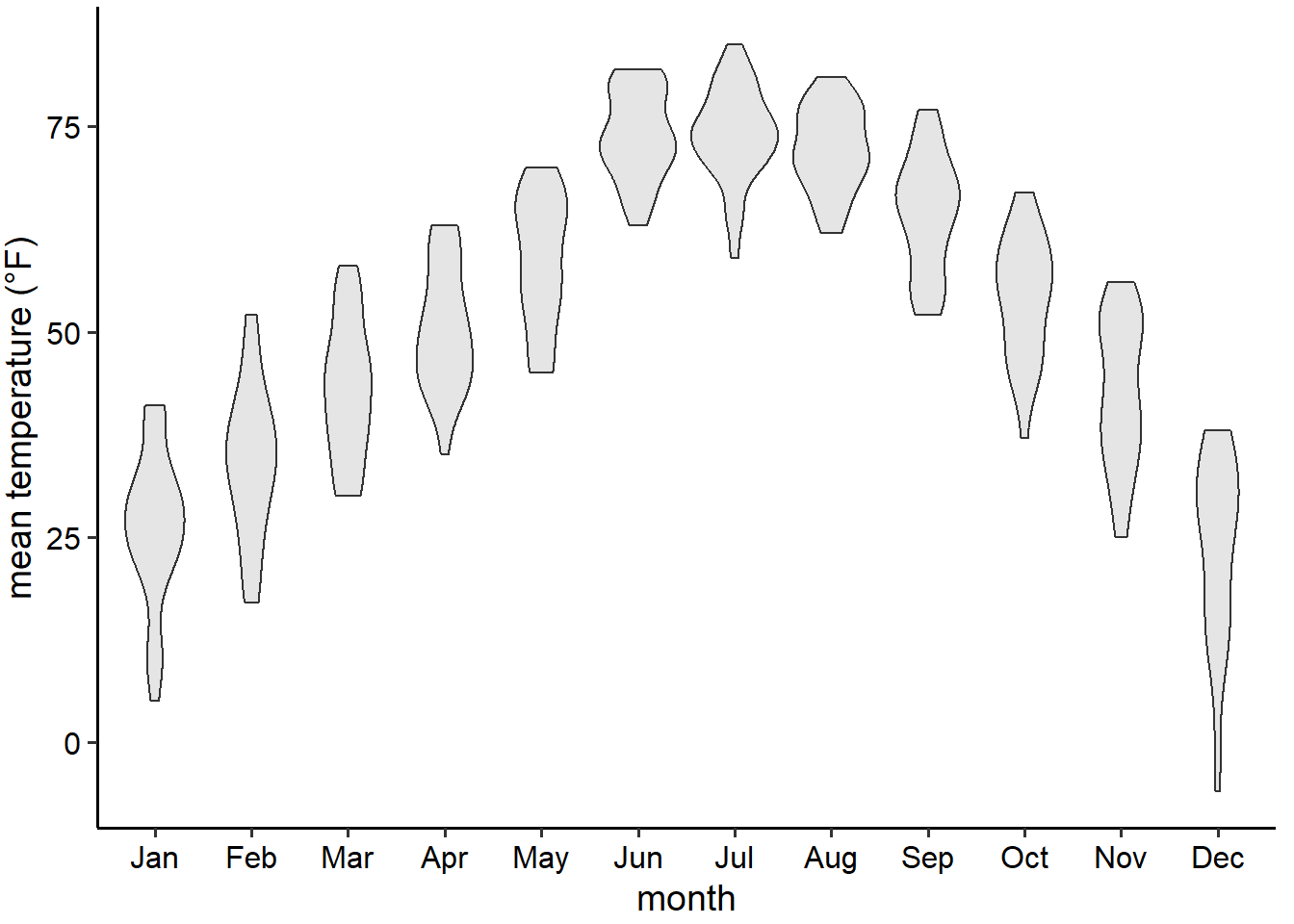

图 32.6: 林肯市2016年气温分布小提琴图

事实上，小提琴图也是不完美的，用的是密度分布图，会造成没有数据点的地方，也会有分布。怎么解决呢？

32.1.4 sina 图

解决办法就是，把原始数据点打上去，

lincoln_points <- lincoln_df %>%
  ggplot(aes(x = month_short, y = `Mean Temperature [F]`)) +
  geom_point(size = 0.75) +
  xlab("month") +
  ylab("mean temperature (°F)") +
  theme_classic(base_size = 14) +
  theme(
    axis.text = element_text(color = "black", size = 12),
    plot.margin = margin(3, 7, 3, 1.5)
  )

lincoln_points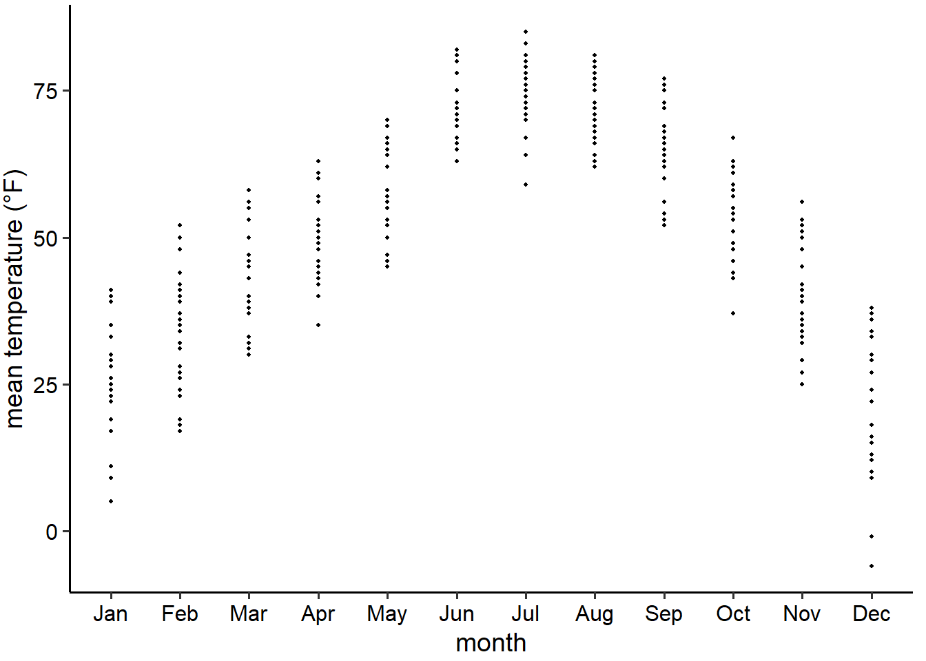

图 32.7: 林肯市2016年气温分布散点图

但问题又来了，这样会有大量重叠的点。有时候会采用透明度的办法，即给每个点设置透明度，某个位置颜色越深，说明这个位置重叠的越多。当然，最好的办法是，给每个点增加一个随机的很小的“偏移”，即抖散图。

lincoln_jitter <- lincoln_df %>%
  ggplot(aes(x = month_short, y = `Mean Temperature [F]`)) +
  geom_point(position = position_jitter(width = .15, height = 0, seed = 320), size = 0.75) +
  xlab("month") +
  ylab("mean temperature (°F)") +
  theme_classic(base_size = 14) +
  theme(
    axis.text = element_text(
      color = "black",
      size = 12
    ),
    plot.margin = margin(3, 7, 3, 1.5)
  )

lincoln_jitter

图 32.8: 林肯市2016年气温分布抖散图

于是，（小提琴图 + 抖散图）= sina 图，这样既可以看到原始的点，又可以看到统计分布，见图 32.9.

lincoln_sina <- lincoln_df %>%
  ggplot(aes(x = month_short, y = `Mean Temperature [F]`)) +
  geom_violin(color = "transparent", fill = "gray90") +
  # dviz.supp::stat_sina(size = 0.85) +
  geom_jitter(width = 0.25, size = 0.85) +
  xlab("month") +
  ylab("mean temperature (°F)") +
  theme_classic(base_size = 14) +
  theme(
    axis.text = element_text(
      color = "black",
      size = 12
    ),
    plot.margin = margin(3, 7, 3, 1.5)
  )

lincoln_sina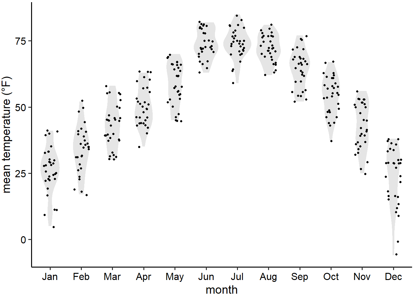

图 32.9: 林肯市2016年气温分布 sina 图

32.1.5 山峦图

前面的图，分组变量（月份）是顺着x轴，这里介绍的山峦图（重山叠叠的感觉）分组变量是顺着y轴，这种图，在画不同时间的分布图的时候，效果非常不错。比如图 32.10，展示气温分布的山峦图。同样，图中很直观地展示了11月份的气温分布有两个峰值。

bandwidth <- 3.4

lincoln_df %>%
  ggplot(aes(x = `Mean Temperature [F]`, y = `Month`)) +
  geom_density_ridges(
    scale = 3, rel_min_height = 0.01,
    bandwidth = bandwidth, fill = colorspace::lighten("#56B4E9", .3), color = "white"
  ) +
  scale_x_continuous(
    name = "mean temperature (°F)",
    expand = c(0, 0), breaks = c(0, 25, 50, 75)
  ) +
  scale_y_discrete(name = NULL, expand = c(0, .2, 0, 2.6)) +
  theme_minimal(base_size = 14) +
  theme(
    axis.text = element_text(color = "black", size = 12),
    axis.text.y = element_text(vjust = 0),
    plot.margin = margin(3, 7, 3, 1.5)
  )

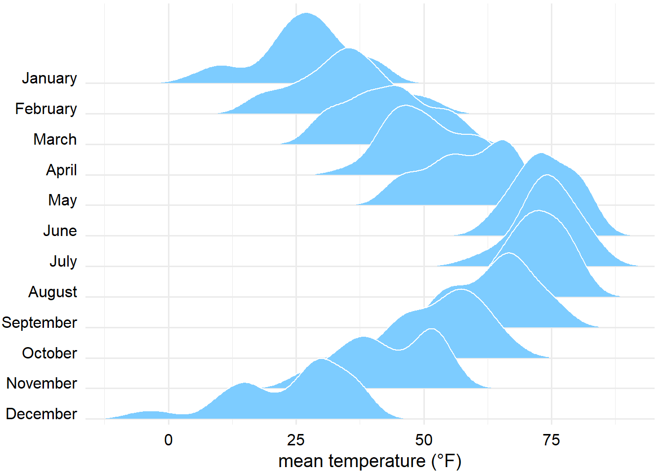
图 32.10: 林肯市2016年气温分布山峦图

但这种图，也有一个问题，y轴是分组变量，x轴是数据的密度分布，缺少了密度分布的标度（即，缺少了密度图的高度，事实上，小提琴图也有这个毛病），所以这种图不适合比较精确的密度分布展示，但在探索性分析中，比较不同分组的密度分布，可以很方便获取直观的认知感受。

32.1.6 有颜色山峦图

我们看到

温度值越高，x轴坐标越靠右；
温度值越高，颜色更亮；

因此，可以将气温变量映射到位置属性和颜色属性，见图 32.11

bandwidth <- 3.4

lincoln_base <- lincoln_weather %>%
  ggplot(aes(x = `Mean Temperature [F]`, y = `Month`, fill = ..x..)) +
  geom_density_ridges_gradient(
    scale = 3, rel_min_height = 0.01, bandwidth = bandwidth,
    color = "black", size = 0.25
  ) +
  scale_x_continuous(
    name = "mean temperature (°F)",
    expand = c(0, 0), breaks = c(0, 25, 50, 75), labels = NULL
  ) +
  scale_y_discrete(name = NULL, expand = c(0, .2, 0, 2.6)) +
  colorspace::scale_fill_continuous_sequential(
    palette = "Heat",
    l1 = 20, l2 = 100, c2 = 0,
    rev = FALSE
  ) +
  guides(fill = "none") +
  theme_minimal(base_size = 14) +
  theme(
    axis.text = element_text(color = "black", size = 12),
    axis.text.y = element_text(vjust = 0),
    plot.margin = margin(3, 7, 3, 1.5)
  )


# x axis labels
temps <- data.frame(temp = c(0, 25, 50, 75))

# calculate corrected color ranges
# stat_joy uses the +/- 3*bandwidth calculation internally
tmin <- min(lincoln_weather$`Mean Temperature [F]`) - 3 * bandwidth
tmax <- max(lincoln_weather$`Mean Temperature [F]`) + 3 * bandwidth

xax <- axis_canvas(lincoln_base, axis = "x", ylim = c(0, 2)) +
  geom_ridgeline_gradient(
    data = data.frame(temp = seq(tmin, tmax, length.out = 100)),
    aes(x = temp, y = 1.1, height = .9, fill = temp),
    color = "transparent"
  ) +
  geom_text(
    data = temps, aes(x = temp, label = temp),
    color = "black", 
    y = 0.9, hjust = 0.5, vjust = 1, size = 14 / .pt
  ) +
  colorspace::scale_fill_continuous_sequential(
    palette = "Heat",
    l1 = 20, l2 = 100, c2 = 0,
    rev = FALSE
  )

## Warning: The dot-dot notation (`..x..`) was deprecated in ggplot2 3.4.0.
## ℹ Please use `after_stat(x)` instead.
## This warning is displayed once every 8 hours.
## Call `lifecycle::last_lifecycle_warnings()` to see where this warning was
## generated.

lincoln_final <- cowplot::insert_xaxis_grob(lincoln_base, xax, position = "bottom", height = unit(0.1, "null"))

ggdraw(lincoln_final)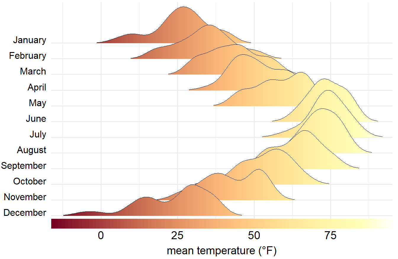

图 32.11: 林肯市2016年气温分布山峦图（颜色越亮，温度越高）

32.2 简单回顾

32.3 说明

本章的数据和代码来源于《Fundamentals of Data Visualization》的第9章和第20章。感谢Claus O. Wilke为大家写了这本非常好的书。

31 ggplot2之延迟映射

33 ggplot2之让你的数据骚动起来