第 78 章 探索性数据分析-诺奖获得者
探索性数据分析(exporatory data analysis)是各种知识的综合运用。本章通过一个案例,讲解探索性数据分析的基本思路,也算是对前面几章内容的一次总结复习。

78.3 导入数据
df <- read_csv("./demo_data/nobel_winners.csv")
df
## # A tibble: 969 × 18
## prize_year category prize motivation prize_share laureate_id laureate_type
## <dbl> <chr> <chr> <chr> <chr> <dbl> <chr>
## 1 1901 Chemistry The N… "\"in rec… 1/1 160 Individual
## 2 1901 Literature The N… "\"in spe… 1/1 569 Individual
## 3 1901 Medicine The N… "\"for hi… 1/1 293 Individual
## 4 1901 Peace The N… <NA> 1/2 462 Individual
## 5 1901 Peace The N… <NA> 1/2 463 Individual
## 6 1901 Physics The N… "\"in rec… 1/1 1 Individual
## 7 1902 Chemistry The N… "\"in rec… 1/1 161 Individual
## 8 1902 Literature The N… "\"the gr… 1/1 571 Individual
## 9 1902 Medicine The N… "\"for hi… 1/1 294 Individual
## 10 1902 Peace The N… <NA> 1/2 464 Individual
## # ℹ 959 more rows
## # ℹ 11 more variables: full_name <chr>, birth_date <date>, birth_city <chr>,
## # birth_country <chr>, gender <chr>, organization_name <chr>,
## # organization_city <chr>, organization_country <chr>, death_date <date>,
## # death_city <chr>, death_country <chr>如果是xlsx格式
readxl::read_excel("myfile.xlsx")如果是csv格式
readr::read_csv("myfile.csv")这里有个小小的提示:
- 路径(包括文件名), 不要用中文和空格
- 数据框中变量,也不要有中文和空格(可用下划线代替空格)
78.4 数据结构
一行就是一个诺奖获得者的记录? 确定?
缺失值及其处理
## # A tibble: 1 × 18
##   prize_year category prize motivation prize_share laureate_id laureate_type
##        <int>    <int> <int>      <int>       <int>       <int>         <int>
## 1          0        0     0         88           0           0             0
## # ℹ 11 more variables: full_name <int>, birth_date <int>, birth_city <int>,
## #   birth_country <int>, gender <int>, organization_name <int>,
## #   organization_city <int>, organization_country <int>, death_date <int>,
## #   death_city <int>, death_country <int>
性别缺失怎么造成的?
## # A tibble: 2 × 2
##   laureate_type     n
##   <chr>         <int>
## 1 Individual      939
## 2 Organization     30
78.5 我们想探索哪些问题?
你想关心哪些问题,可能是
- 每个学科颁过多少次奖?
- 这些大神都是哪个年代的人?
- 性别比例
- 平均年龄和获奖数量
- 最年轻的诺奖获得者是谁?
- 中国诺奖获得者有哪些?
- 得奖的时候多大年龄?
- 获奖者所在国家的经济情况?
- 有大神多次获得诺贝尔奖,而且在不同科学领域获奖?
- 出生地分布?工作地分布?迁移模式?
- GDP经济与诺奖模型?
- 诺奖分享情况?
78.6 每个学科颁过多少次奖
## # A tibble: 6 × 2
##   category       n
##   <chr>      <int>
## 1 Chemistry    194
## 2 Economics     83
## 3 Literature   113
## 4 Medicine     227
## 5 Peace        130
## 6 Physics      222
df %>%
count(category) %>%
ggplot(aes(x = category, y = n, fill = category)) +
geom_col() +
geom_text(aes(label = n), vjust = -0.25) +
theme(legend.position = "none")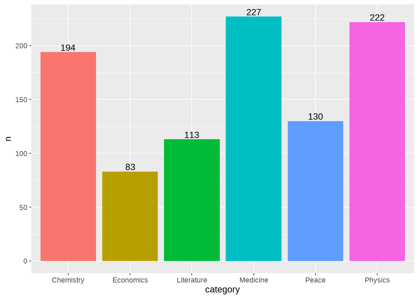
df %>%
  count(category) %>%
  ggplot(aes(x = fct_reorder(category, n), y = n, fill = category)) +
  geom_col() +
  geom_text(aes(label = n), vjust = -0.25) +
  labs(title = "Number of Nobel prizes in different disciplines") +
  theme(legend.position = "none")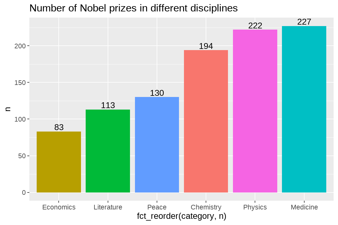
也可以使用别人定义好的配色方案
library(ggthemr) # install.packages("devtools")
# devtools::install_github('cttobin/ggthemr')
ggthemr("dust")

df %>%
  count(category) %>%
  ggplot(aes(x = fct_reorder(category, n), y = n, fill = category)) +
  geom_col() +
  labs(title = "Number of Nobel prizes in different disciplines") +
  theme(legend.position = "none")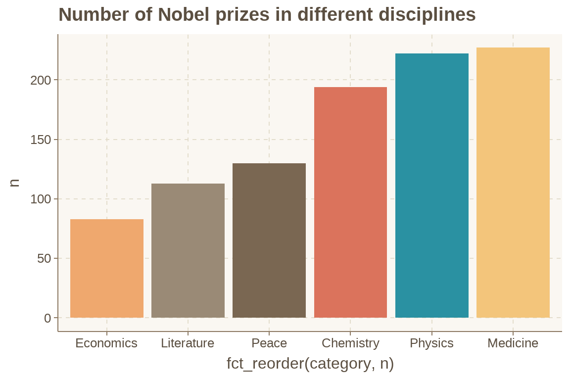
这个配色方案感觉挺好看的呢,比较适合我这种又挑剔又懒惰的人。
当然,也可以自己DIY,或者使用配色网站的主题方案(https://learnui.design/tools/data-color-picker.html#palette)
df %>%
  count(category) %>%
  ggplot(aes(x = fct_reorder(category, n), y = n)) +
  geom_col(fill = c("#003f5c", "#444e86", "#955196", "#dd5182", "#ff6e54", "#ffa600")) +
  labs(title = "Number of Nobel prizes in different disciplines") +
  theme(legend.position = "none")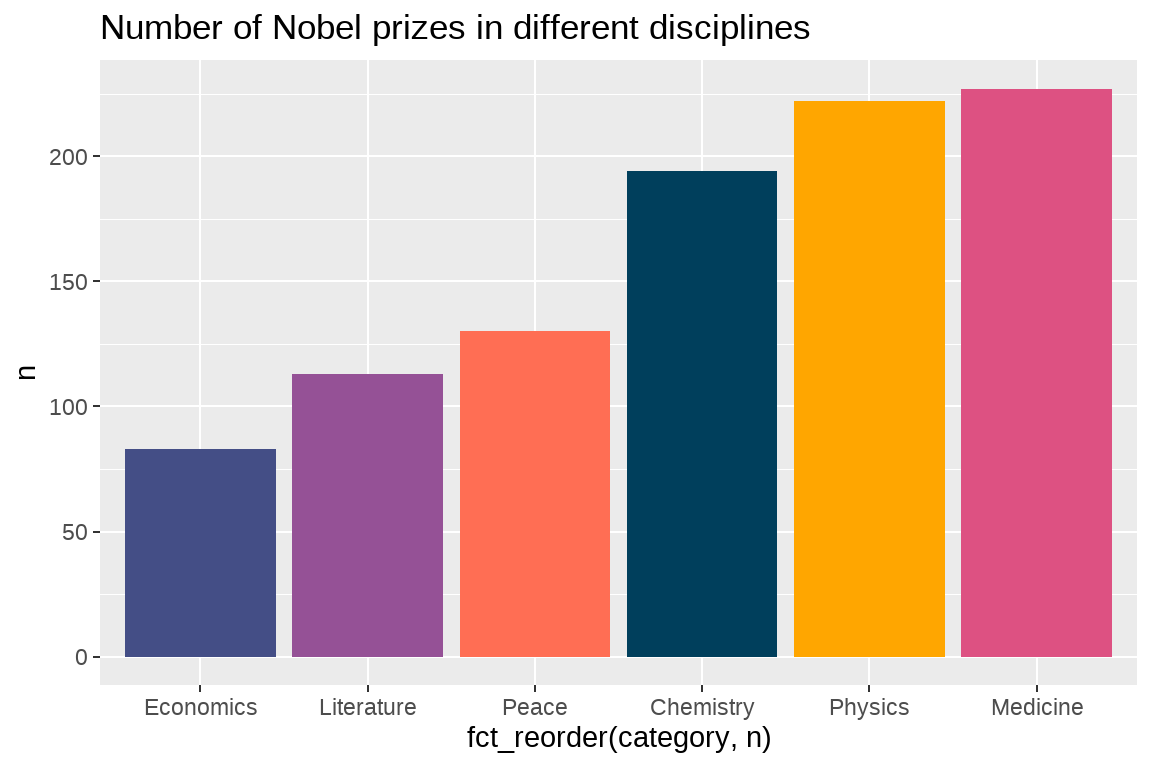
让图骚动起来吧
library(gganimate) # install.packages("gganimate", dependencies = T)

df %>%
  count(category) %>%
  mutate(category = fct_reorder(category, n)) %>%
  ggplot(aes(x = category, y = n)) +
  geom_text(aes(label = n), vjust = -0.25) +
  geom_col(fill = c("#003f5c", "#444e86", "#955196", "#dd5182", "#ff6e54", "#ffa600")) +
  labs(title = "Number of Nobel prizes in different disciplines") +
  theme(legend.position = "none") +
  transition_states(category) +
  shadow_mark(past = TRUE)
和ggplot2的分面一样,动态图可以增加数据展示的维度。
78.7 看看我们伟大的祖国
## # A tibble: 12 × 3
##    full_name              prize_year category
##    <chr>                       <dbl> <chr>
##  1 Walter Houser Brattain       1956 Physics
##  2 Chen Ning Yang               1957 Physics
##  3 Tsung-Dao (T.D.) Lee         1957 Physics
##  4 Edmond H. Fischer            1992 Medicine
##  5 Daniel C. Tsui               1998 Physics
##  6 Gao Xingjian                 2000 Literature
##  7 Charles Kuen Kao             2009 Physics
##  8 Charles Kuen Kao             2009 Physics
##  9 Ei-ichi Negishi              2010 Chemistry
## 10 Liu Xiaobo                   2010 Peace
## 11 Mo Yan                       2012 Literature
## 12 Youyou Tu                    2015 Medicine
我们发现获奖者有多个地址,就会有重复的情况,比如 Charles Kuen Kao在2009年Physics有两次,为什么重复计数了呢?
下面我们去重吧, 去重可以用distinct()函数
dt <- tibble::tribble(
  ~x, ~y, ~z,
  1, 1, "a",
  1, 1, "b",
  1, 2, "c",
  1, 2, "d"
)

dt
## # A tibble: 4 × 3
## x y z
## <dbl> <dbl> <chr>
## 1 1 1 a
## 2 1 1 b
## 3 1 2 c
## 4 1 2 ddt %>% distinct_at(vars(x), .keep_all = T)## # A tibble: 1 × 3
## x y z
## <dbl> <dbl> <chr>
## 1 1 1 adt %>% distinct_at(vars(x, y), .keep_all = T)## # A tibble: 2 × 3
## x y z
## <dbl> <dbl> <chr>
## 1 1 1 a
## 2 1 2 cnobel_winners <- df %>%
mutate_if(is.character, tolower) %>%
distinct_at(vars(full_name, prize_year, category), .keep_all = TRUE) %>%
mutate(
decade = 10 * (prize_year %/% 10),
prize_age = prize_year - year(birth_date)
)
nobel_winners## # A tibble: 911 × 20
## prize_year category prize motivation prize_share laureate_id laureate_type
## <dbl> <chr> <chr> <chr> <chr> <dbl> <chr>
## 1 1901 chemistry the n… "\"in rec… 1/1 160 individual
## 2 1901 literature the n… "\"in spe… 1/1 569 individual
## 3 1901 medicine the n… "\"for hi… 1/1 293 individual
## 4 1901 peace the n… <NA> 1/2 462 individual
## 5 1901 peace the n… <NA> 1/2 463 individual
## 6 1901 physics the n… "\"in rec… 1/1 1 individual
## 7 1902 chemistry the n… "\"in rec… 1/1 161 individual
## 8 1902 literature the n… "\"the gr… 1/1 571 individual
## 9 1902 medicine the n… "\"for hi… 1/1 294 individual
## 10 1902 peace the n… <NA> 1/2 464 individual
## # ℹ 901 more rows
## # ℹ 13 more variables: full_name <chr>, birth_date <date>, birth_city <chr>,
## # birth_country <chr>, gender <chr>, organization_name <chr>,
## # organization_city <chr>, organization_country <chr>, death_date <date>,
## # death_city <chr>, death_country <chr>, decade <dbl>, prize_age <dbl>这是时候,我们才对数据有了一个初步的了解
再来看看我的祖国
nobel_winners %>%
  dplyr::filter(birth_country == "china") %>%
  dplyr::select(full_name, prize_year, category)
## # A tibble: 11 × 3
## full_name prize_year category
## <chr> <dbl> <chr>
## 1 walter houser brattain 1956 physics
## 2 chen ning yang 1957 physics
## 3 tsung-dao (t.d.) lee 1957 physics
## 4 edmond h. fischer 1992 medicine
## 5 daniel c. tsui 1998 physics
## 6 gao xingjian 2000 literature
## 7 charles kuen kao 2009 physics
## 8 ei-ichi negishi 2010 chemistry
## 9 liu xiaobo 2010 peace
## 10 mo yan 2012 literature
## 11 youyou tu 2015 medicine78.8 哪些大神多次获得诺贝尔奖
## # A tibble: 904 × 2
##    full_name                                                                   n
##    <chr>                                                                   <int>
##  1 comité international de la croix rouge (international committee of the…     3
##  2 frederick sanger                                                            2
##  3 john bardeen                                                                2
##  4 linus carl pauling                                                          2
##  5 marie curie, née sklodowska                                                 2
##  6 office of the united nations high commissioner for refugees (unhcr)         2
##  7 a. michael spence                                                           1
##  8 aage niels bohr                                                             1
##  9 aaron ciechanover                                                           1
## 10 aaron klug                                                                  1
## # ℹ 894 more rows
nobel_winners %>%
group_by(full_name) %>%
mutate(
number_prize = n(),
number_cateory = n_distinct(category)
) %>%
arrange(desc(number_prize), full_name) %>%
dplyr::filter(number_cateory == 2)## # A tibble: 4 × 22
## # Groups: full_name [2]
## prize_year category prize motivation prize_share laureate_id laureate_type
## <dbl> <chr> <chr> <chr> <chr> <dbl> <chr>
## 1 1954 chemistry the nob… "\"for hi… 1/1 217 individual
## 2 1962 peace the nob… <NA> 1/1 217 individual
## 3 1903 physics the nob… "\"in rec… 1/4 6 individual
## 4 1911 chemistry the nob… "\"in rec… 1/1 6 individual
## # ℹ 15 more variables: full_name <chr>, birth_date <date>, birth_city <chr>,
## # birth_country <chr>, gender <chr>, organization_name <chr>,
## # organization_city <chr>, organization_country <chr>, death_date <date>,
## # death_city <chr>, death_country <chr>, decade <dbl>, prize_age <dbl>,
## # number_prize <int>, number_cateory <int>78.9 大神在得奖的时候是多大年龄?
## # A tibble: 6 × 2
##   category   mean_prize_age
##   <chr>               <dbl>
## 1 chemistry            58.0
## 2 economics            67.2
## 3 literature           64.7
## 4 medicine             58.0
## 5 peace                61.4
## 6 physics              55.4
nobel_winners %>%
mutate(category = fct_reorder(category, prize_age, median, na.rm = TRUE)) %>%
ggplot(aes(category, prize_age)) +
geom_point() +
geom_boxplot() +
coord_flip()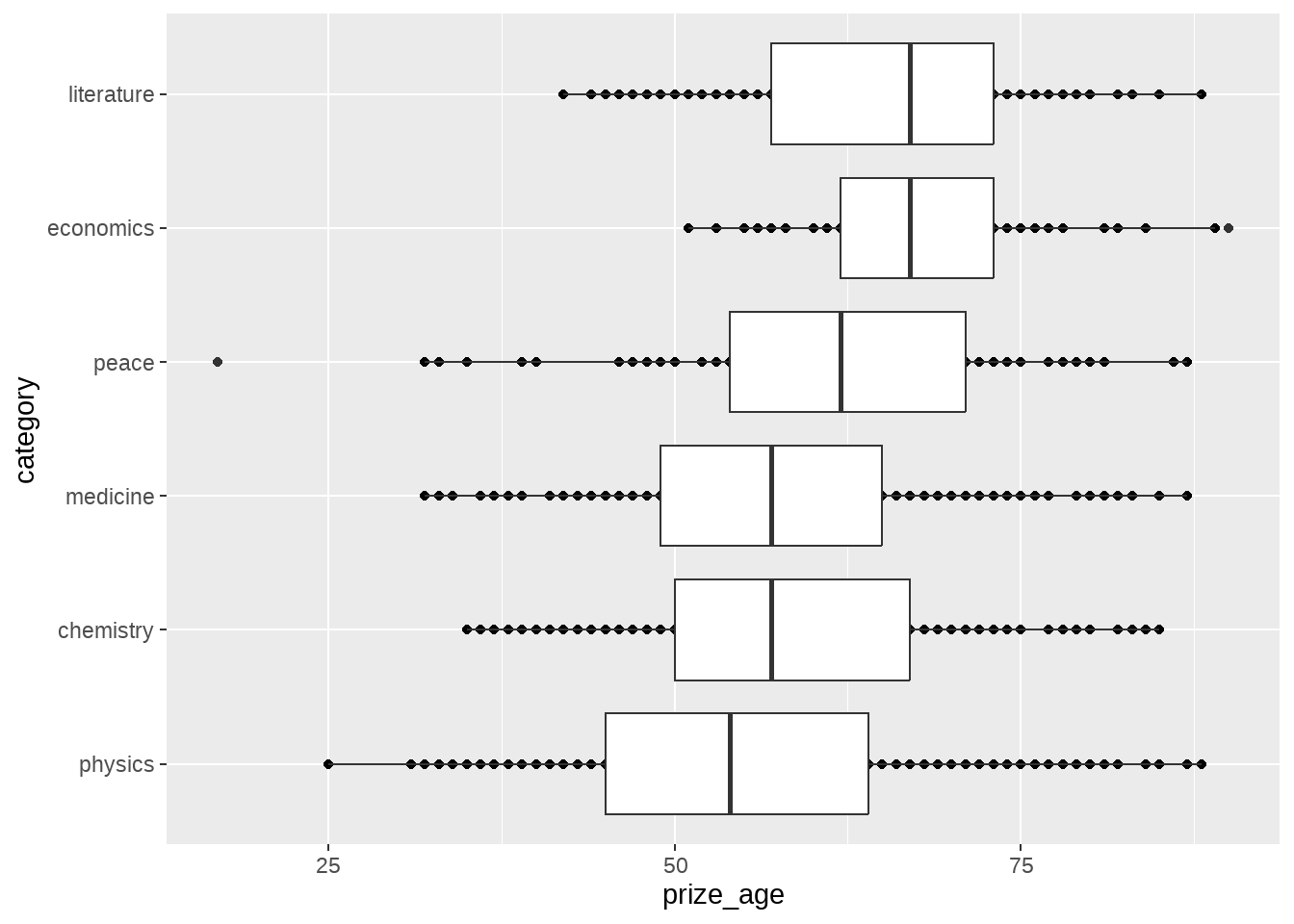
nobel_winners %>%
  dplyr::filter(!is.na(prize_age)) %>%
  group_by(decade, category) %>%
  summarize(
    average_age = mean(prize_age),
    median_age = median(prize_age)
  ) %>%
  ggplot(aes(decade, average_age, color = category)) +
  geom_line()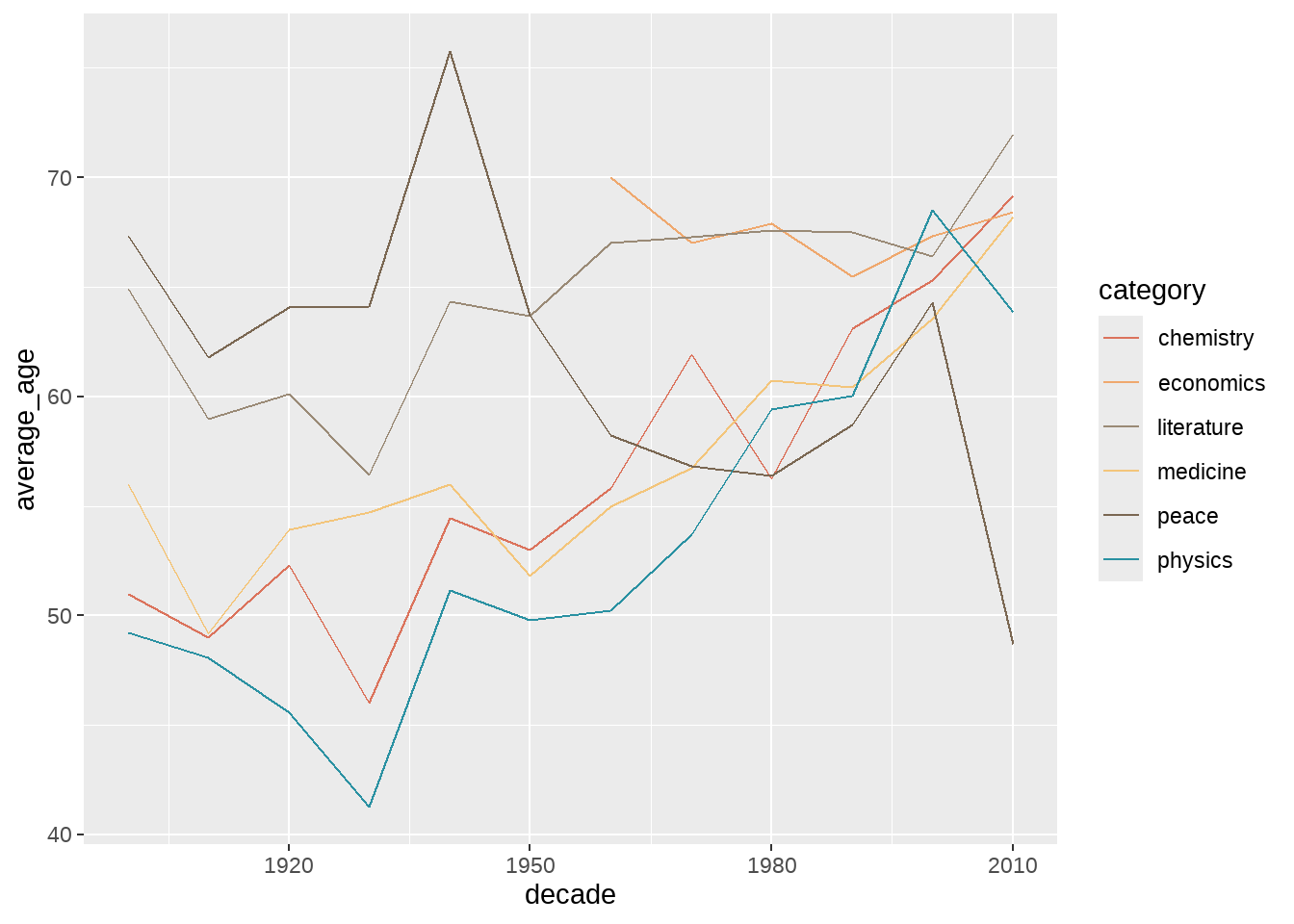
library(ggridges)

nobel_winners %>%
  ggplot(aes(
    x = prize_age,
    y = category,
    fill = category
  )) +
  geom_density_ridges()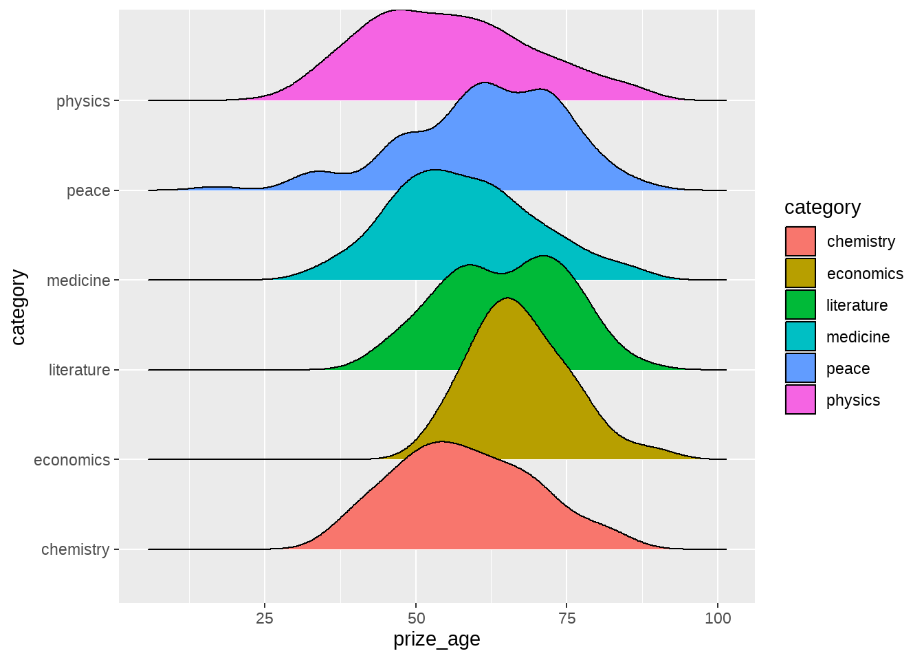
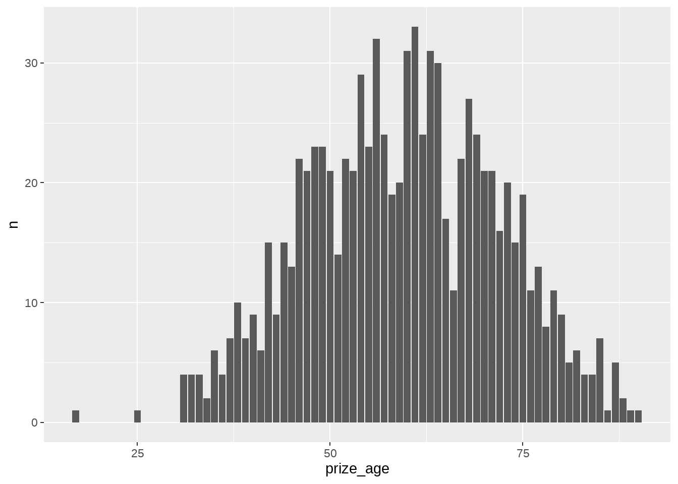
他们60多少岁才得诺奖,大家才23或24岁,还年轻,不用焦虑喔。
nobel_winners %>%

  ggplot(aes(x = prize_age, fill = category, color = category)) +
  geom_density() +
  facet_wrap(vars(category)) +
  theme(legend.position = "none")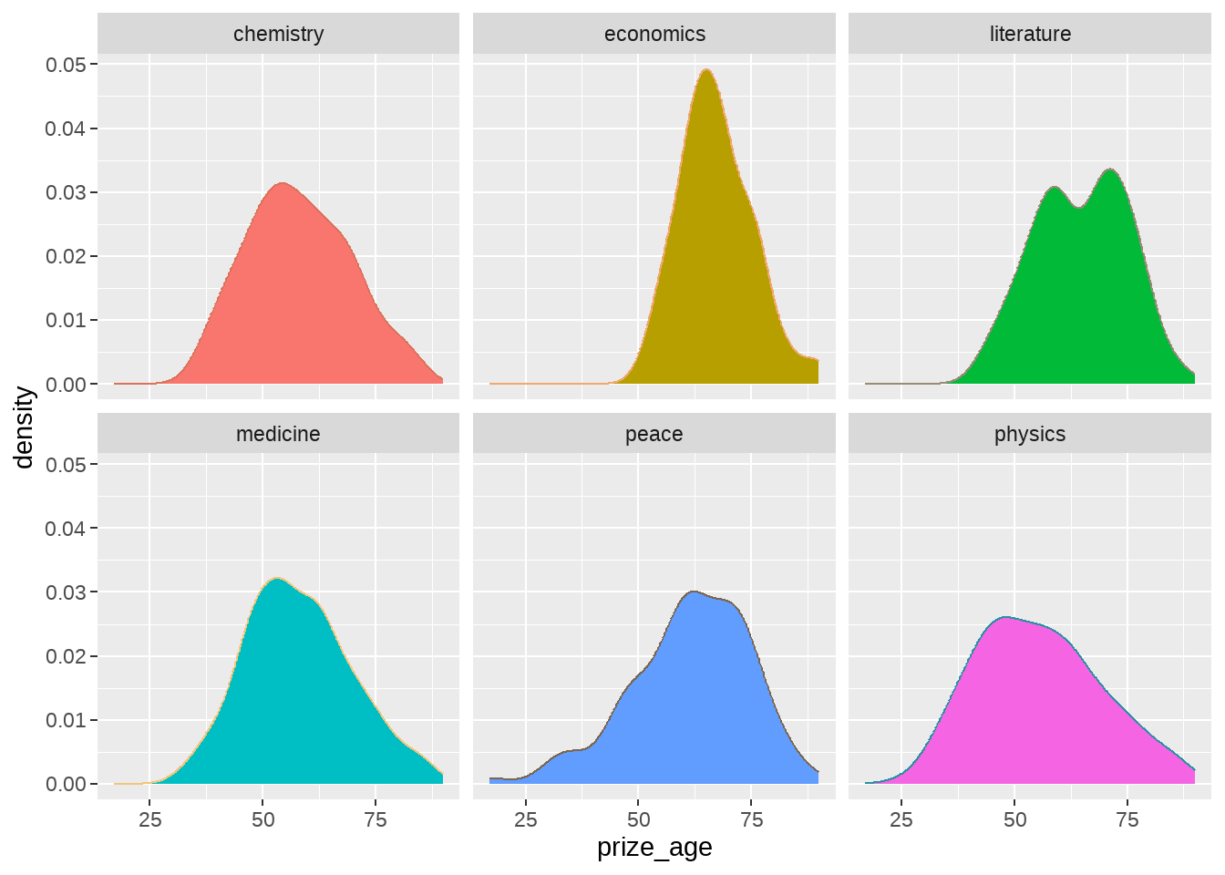
有同学说要一个个的画,至于group_split()函数,下次课在讲
nobel_winners %>%
  group_split(category) %>%
  map(
    ~ ggplot(data = .x, aes(x = prize_age)) +
      geom_density() +
      ggtitle(.x$category)
  )
## [[1]]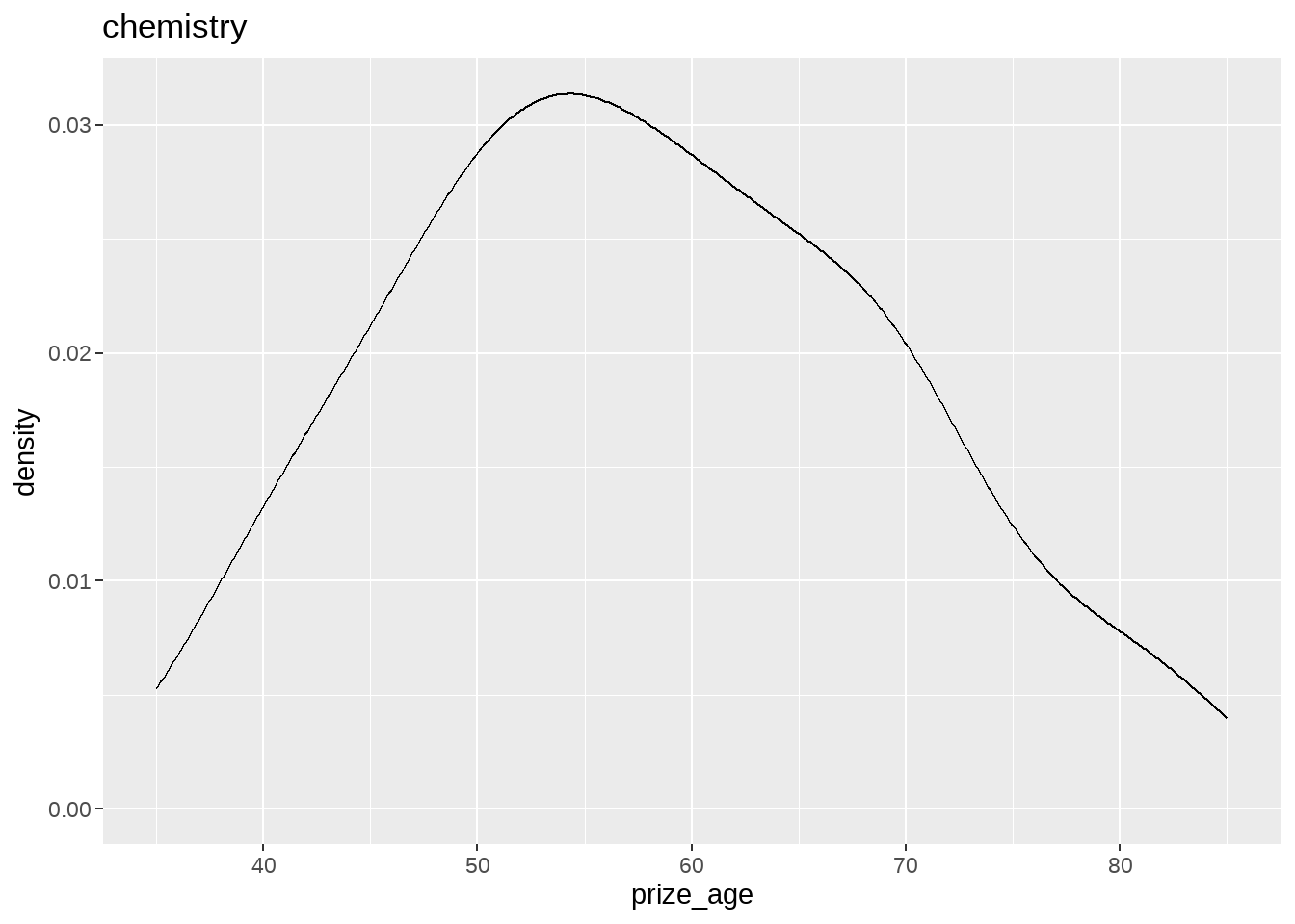
##
## [[2]]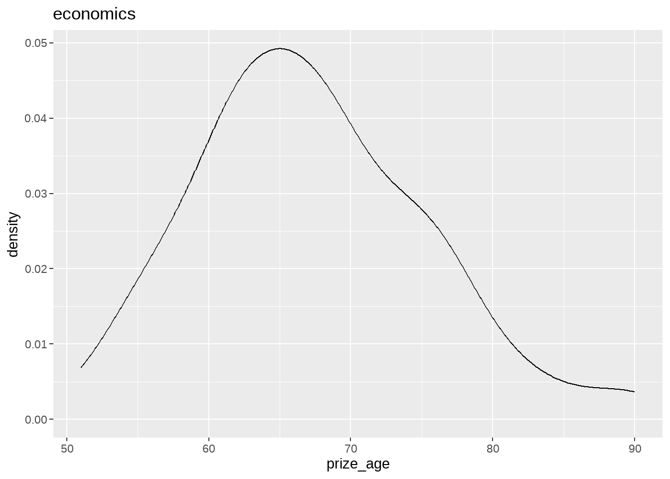
##
## [[3]]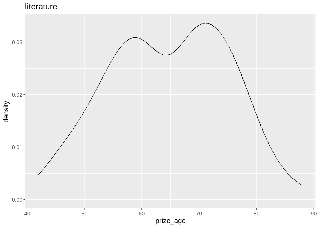
##
## [[4]]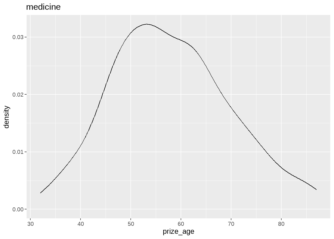
##
## [[5]]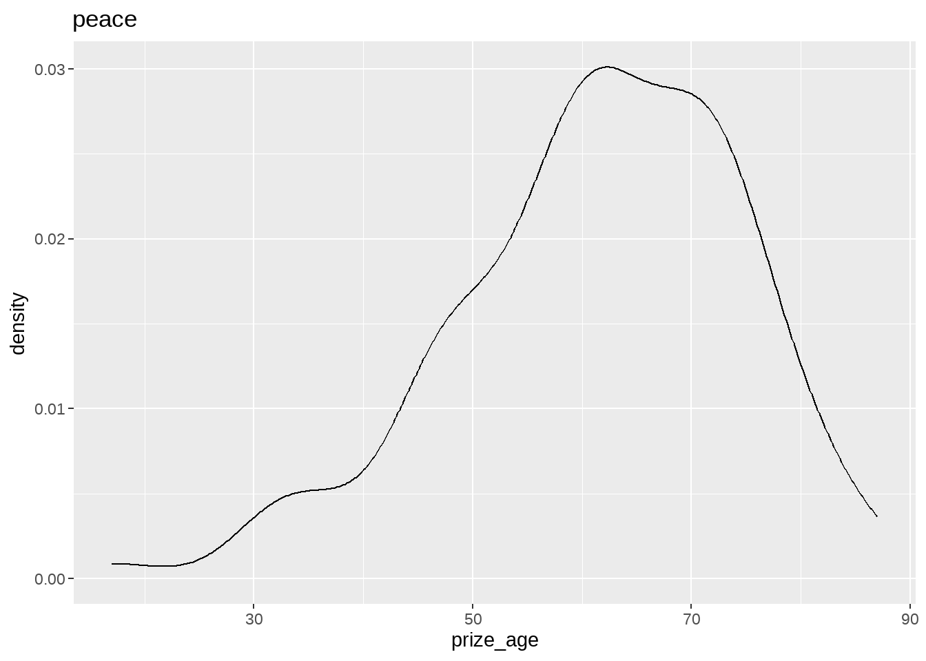
##
## [[6]]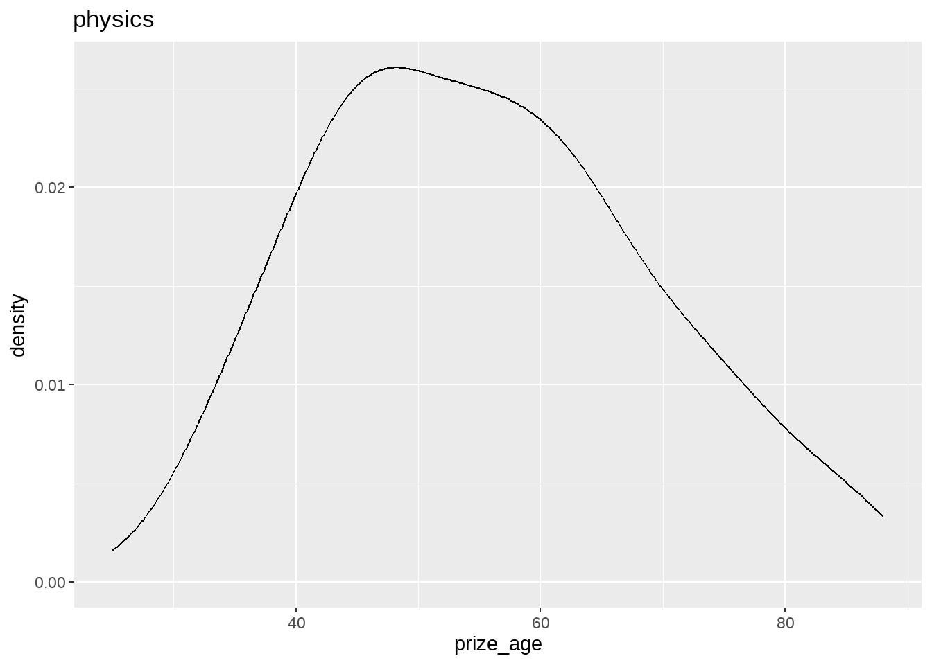
也可以用强大的group_by() + group_map()组合,我们会在第 37 章讲到
78.10 性别比例
nobel_winners %>%
  dplyr::filter(laureate_type == "individual") %>%
  count(category, gender) %>%
  group_by(category) %>%
  mutate(prop = n / sum(n))
## # A tibble: 12 × 4
## # Groups: category [6]
## category gender n prop
## <chr> <chr> <int> <dbl>
## 1 chemistry female 4 0.0229
## 2 chemistry male 171 0.977
## 3 economics female 1 0.0128
## 4 economics male 77 0.987
## 5 literature female 14 0.124
## 6 literature male 99 0.876
## 7 medicine female 12 0.0569
## 8 medicine male 199 0.943
## 9 peace female 14 0.14
## 10 peace male 86 0.86
## 11 physics female 2 0.00980
## 12 physics male 202 0.990各年代性别比例
nobel_winners %>%
  dplyr::filter(laureate_type == "individual") %>%
  # mutate(decade = glue::glue("{round(prize_year - 1, -1)}s")) %>%
  count(decade, category, gender) %>%
  group_by(decade, category) %>%
  mutate(prop = n / sum(n)) %>%
  ggplot(aes(decade, category, fill = prop)) +
  geom_tile(size = 0.7) +
  # geom_text(aes(label = scales::percent(prop, accuracy = .01))) +
  geom_text(aes(label = scales::number(prop, accuracy = .01))) +
  facet_grid(vars(gender)) +
  scale_fill_gradient(low = "#FDF4E9", high = "#834C0D")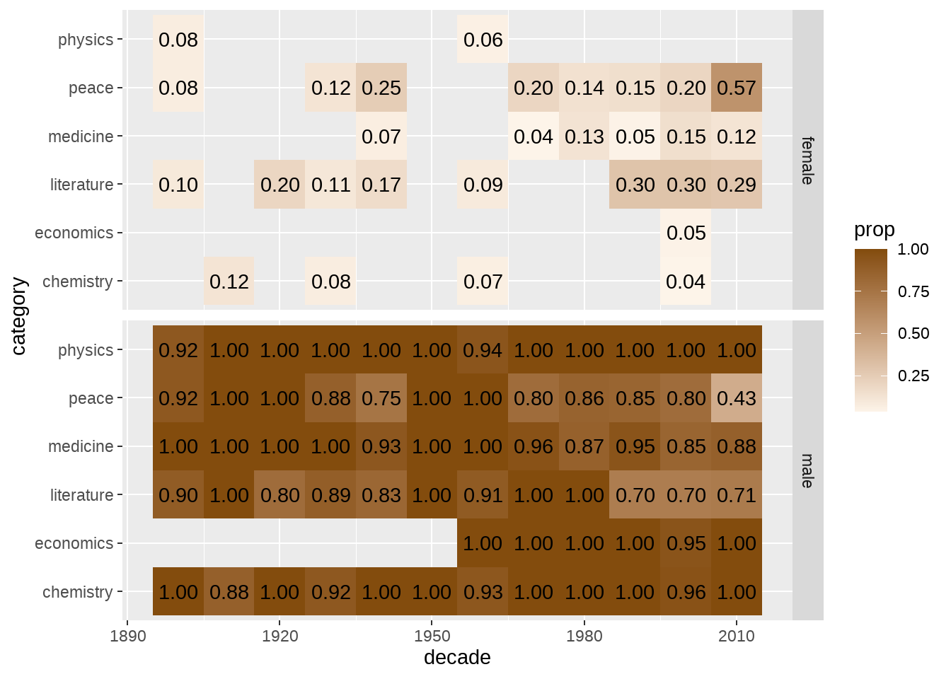
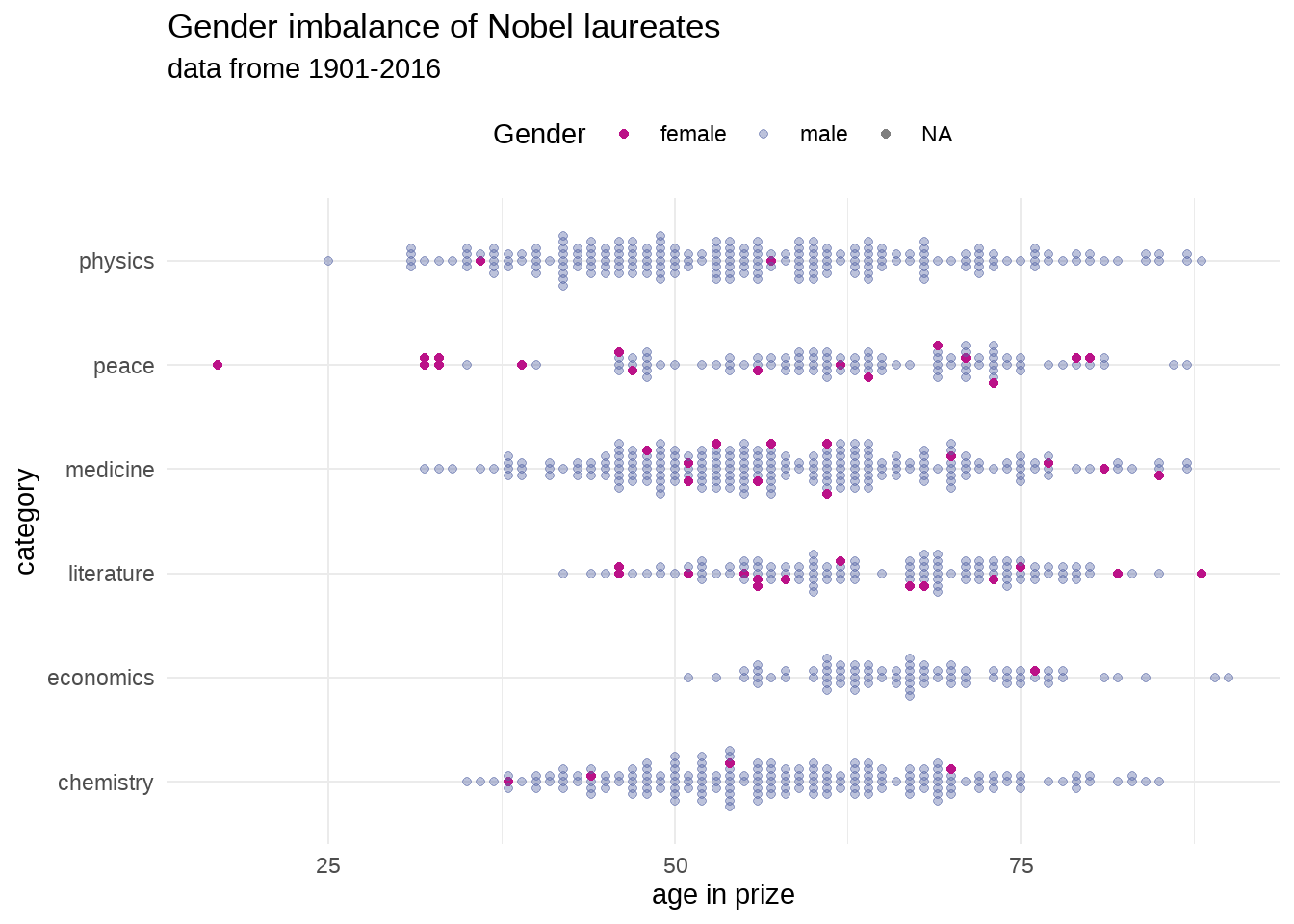
library(ggbeeswarm) # install.packages("ggbeeswarm")

nobel_winners %>%
  ggplot(aes(
    x = category,
    y = prize_age,
    colour = gender,
    alpha = gender
  )) +
  ggbeeswarm::geom_beeswarm() +
  coord_flip() +
  scale_color_manual(values = c("#BB1288", "#5867A6")) +
  scale_alpha_manual(values = c(1, .4)) +
  theme_minimal() +
  theme(legend.position = "top") +
  labs(
    title = "Gender imbalance of Nobel laureates",
    subtitle = "data frome 1901-2016",
    colour = "Gender",
    alpha = "Gender",
    y = "age in prize"
  )
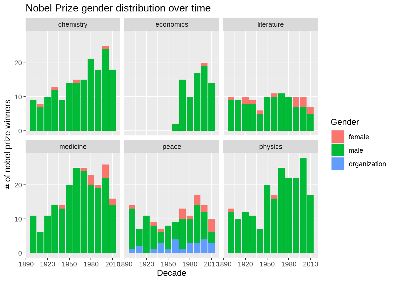
nobel_winners %>%
  count(decade,
    category,
    gender = coalesce(gender, laureate_type)
  ) %>%
  group_by(decade, category) %>%
  mutate(percent = n / sum(n)) %>%
  ggplot(aes(decade, n, fill = gender)) +
  geom_col() +
  facet_wrap(~category) +
  labs(
    x = "Decade",
    y = "# of nobel prize winners",
    fill = "Gender",
    title = "Nobel Prize gender distribution over time"
  )
78.11 这些大神都是哪个年代出生的人?
nobel_winners %>%
  select(category, birth_date) %>%
  mutate(year = floor(year(birth_date) / 10) * 10) %>%
  count(category, year) %>%
  dplyr::filter(!is.na(year)) %>%
  ggplot(aes(x = year, y = n)) +
  geom_col() +
  scale_x_continuous(breaks = seq(1810, 1990, 20)) +
  geom_text(aes(label = n), vjust = -0.25) +
  facet_wrap(vars(category))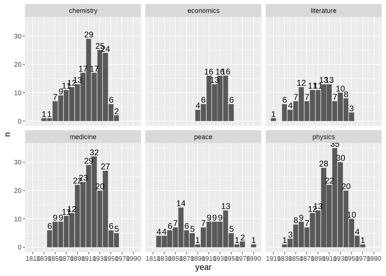
课堂练习,哪位同学能把图弄得好看些?
78.12 最年轻的诺奖获得者?
## # A tibble: 1 × 20
##   prize_year category prize     motivation prize_share laureate_id laureate_type
##        <dbl> <chr>    <chr>     <chr>      <chr>             <dbl> <chr>
## 1       2014 peace    the nobe… "\"for th… 1/2                 914 individual
## # ℹ 13 more variables: full_name <chr>, birth_date <date>, birth_city <chr>,
## #   birth_country <chr>, gender <chr>, organization_name <chr>,
## #   organization_city <chr>, organization_country <chr>, death_date <date>,
## # death_city <chr>, death_country <chr>, decade <dbl>, prize_age <dbl>## # A tibble: 1 × 20
## prize_year category prize motivation prize_share laureate_id laureate_type
## <dbl> <chr> <chr> <chr> <chr> <dbl> <chr>
## 1 2014 peace the nobe… "\"for th… 1/2 914 individual
## # ℹ 13 more variables: full_name <chr>, birth_date <date>, birth_city <chr>,
## # birth_country <chr>, gender <chr>, organization_name <chr>,
## # organization_city <chr>, organization_country <chr>, death_date <date>,
## # death_city <chr>, death_country <chr>, decade <dbl>, prize_age <dbl>## # A tibble: 911 × 20
## prize_year category prize motivation prize_share laureate_id laureate_type
## <dbl> <chr> <chr> <chr> <chr> <dbl> <chr>
## 1 2014 peace the nob… "\"for th… 1/2 914 individual
## 2 1915 physics the nob… "\"for th… 1/2 21 individual
## 3 1932 physics the nob… "\"for th… 1/1 38 individual
## 4 1933 physics the nob… "\"for th… 1/2 40 individual
## 5 1936 physics the nob… "\"for hi… 1/2 43 individual
## 6 1957 physics the nob… "\"for th… 1/2 69 individual
## 7 1923 medicine the nob… "\"for th… 1/2 313 individual
## 8 1961 physics the nob… "\"for hi… 1/2 76 individual
## 9 1976 peace the nob… <NA> 1/2 536 individual
## 10 2011 peace the nob… "\"for th… 1/3 871 individual
## # ℹ 901 more rows
## # ℹ 13 more variables: full_name <chr>, birth_date <date>, birth_city <chr>,
## # birth_country <chr>, gender <chr>, organization_name <chr>,
## # organization_city <chr>, organization_country <chr>, death_date <date>,
## # death_city <chr>, death_country <chr>, decade <dbl>, prize_age <dbl>## # A tibble: 1 × 20
## prize_year category prize motivation prize_share laureate_id laureate_type
## <dbl> <chr> <chr> <chr> <chr> <dbl> <chr>
## 1 2014 peace the nobe… "\"for th… 1/2 914 individual
## # ℹ 13 more variables: full_name <chr>, birth_date <date>, birth_city <chr>,
## # birth_country <chr>, gender <chr>, organization_name <chr>,
## # organization_city <chr>, organization_country <chr>, death_date <date>,
## # death_city <chr>, death_country <chr>, decade <dbl>, prize_age <dbl>78.13 平均年龄和获奖数量
df1 <- nobel_winners %>%
  group_by(category) %>%
  summarise(
    mean_prise_age = mean(prize_age, na.rm = T),
    total_num = n()
  )
df1
## # A tibble: 6 × 3
## category mean_prise_age total_num
## <chr> <dbl> <int>
## 1 chemistry 58.0 175
## 2 economics 67.2 78
## 3 literature 64.7 113
## 4 medicine 58.0 211
## 5 peace 61.4 130
## 6 physics 55.4 204df1 %>%
ggplot(aes(mean_prise_age, total_num)) +
geom_point(aes(color = category)) +
geom_smooth(method = lm, se = FALSE)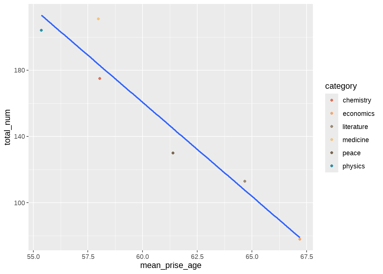
78.14 出生地与工作地分布
nobel_winners_clean <- nobel_winners %>%
  mutate_at(
    vars(birth_country, death_country),
    ~ ifelse(str_detect(., "\\("), str_extract(., "(?<=\\().*?(?=\\))"), .)
  ) %>%
  mutate_at(
    vars(birth_country, death_country),
    ~ case_when(
      . == "scotland" ~ "united kingdom",
      . == "northern ireland" ~ "united kingdom",
      str_detect(., "czech") ~ "czechia",
      str_detect(., "germany") ~ "germany",
      TRUE ~ .
    )
  ) %>%
select(full_name, prize_year, category, birth_date, birth_country, gender, organization_name, organization_country, death_country)## # A tibble: 45 × 2
## death_country n
## <chr> <int>
## 1 <NA> 329
## 2 united states of america 203
## 3 united kingdom 79
## 4 germany 56
## 5 france 51
## 6 sweden 28
## 7 switzerland 26
## 8 italy 14
## 9 russia 11
## 10 spain 10
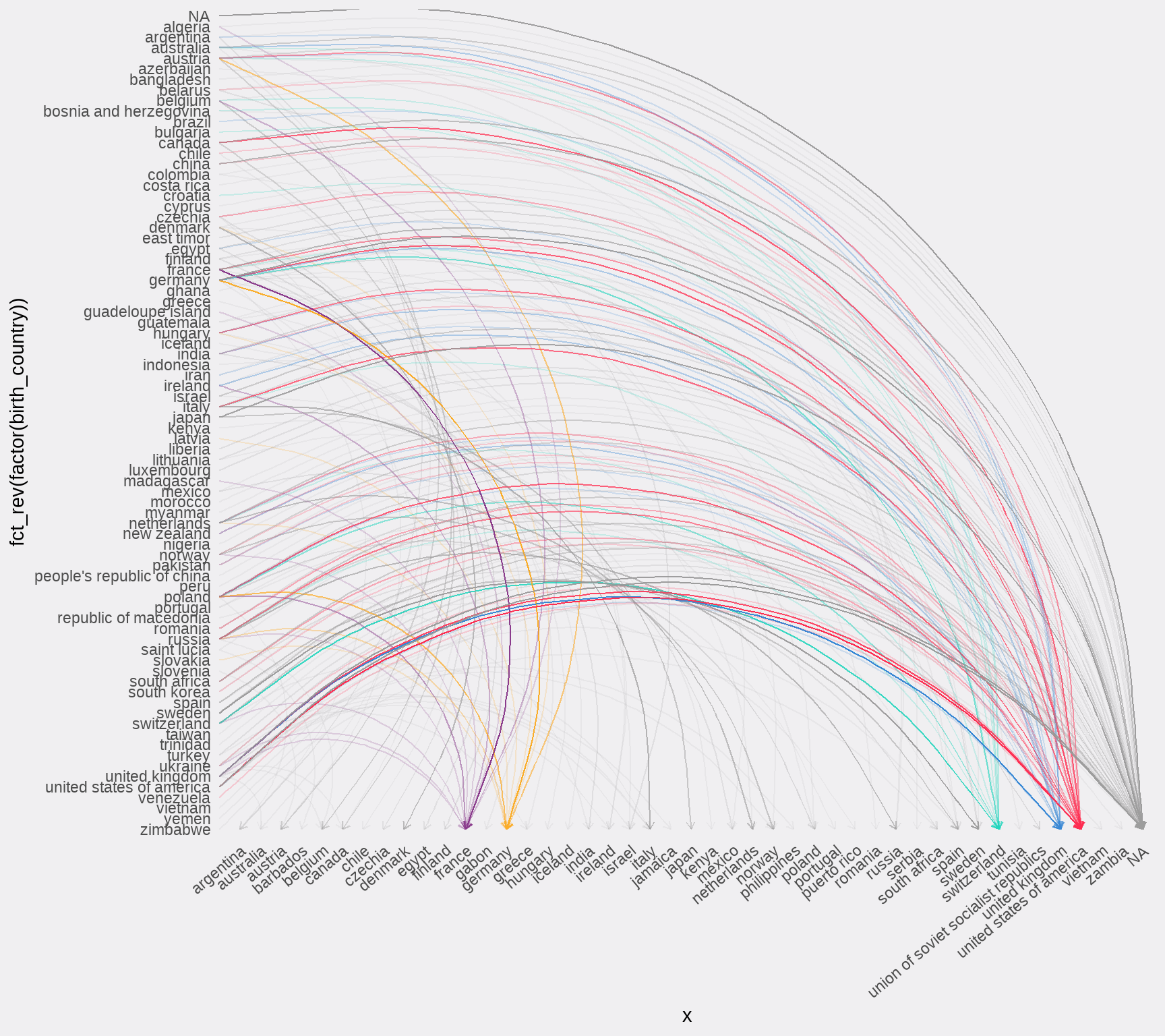
## # ℹ 35 more rows78.15 迁移模式
nobel_winners_clean %>%
  mutate(
    colour = case_when(
      death_country == "united states of america" ~ "#FF2B4F",
      death_country == "germany" ~ "#fcab27",
      death_country == "united kingdom" ~ "#3686d3",
      death_country == "france" ~ "#88398a",
      death_country == "switzerland" ~ "#20d4bc",
      TRUE ~ "gray60"
    )
  ) %>%
  ggplot(aes(
    x = 0,
    y = fct_rev(factor(birth_country)),
    xend = death_country,
    yend = 1,
    colour = colour,
    alpha = (colour != "gray60")
  )) +
  geom_curve(
    curvature = -0.5,
    arrow = arrow(length = unit(0.01, "npc"))
  ) +
  scale_x_discrete() +
  scale_y_discrete() +
  scale_color_identity() +
  scale_alpha_manual(values = c(0.1, 0.2), guide = F) +
  scale_size_manual(values = c(0.1, 0.4), guide = F) +
  theme_minimal() +
  theme(
    panel.grid = element_blank(),
    plot.background = element_rect(fill = "#F0EFF1", colour = "#F0EFF1"),
    legend.position = "none",
    axis.text.x = element_text(angle = 40, hjust = 1)
  )
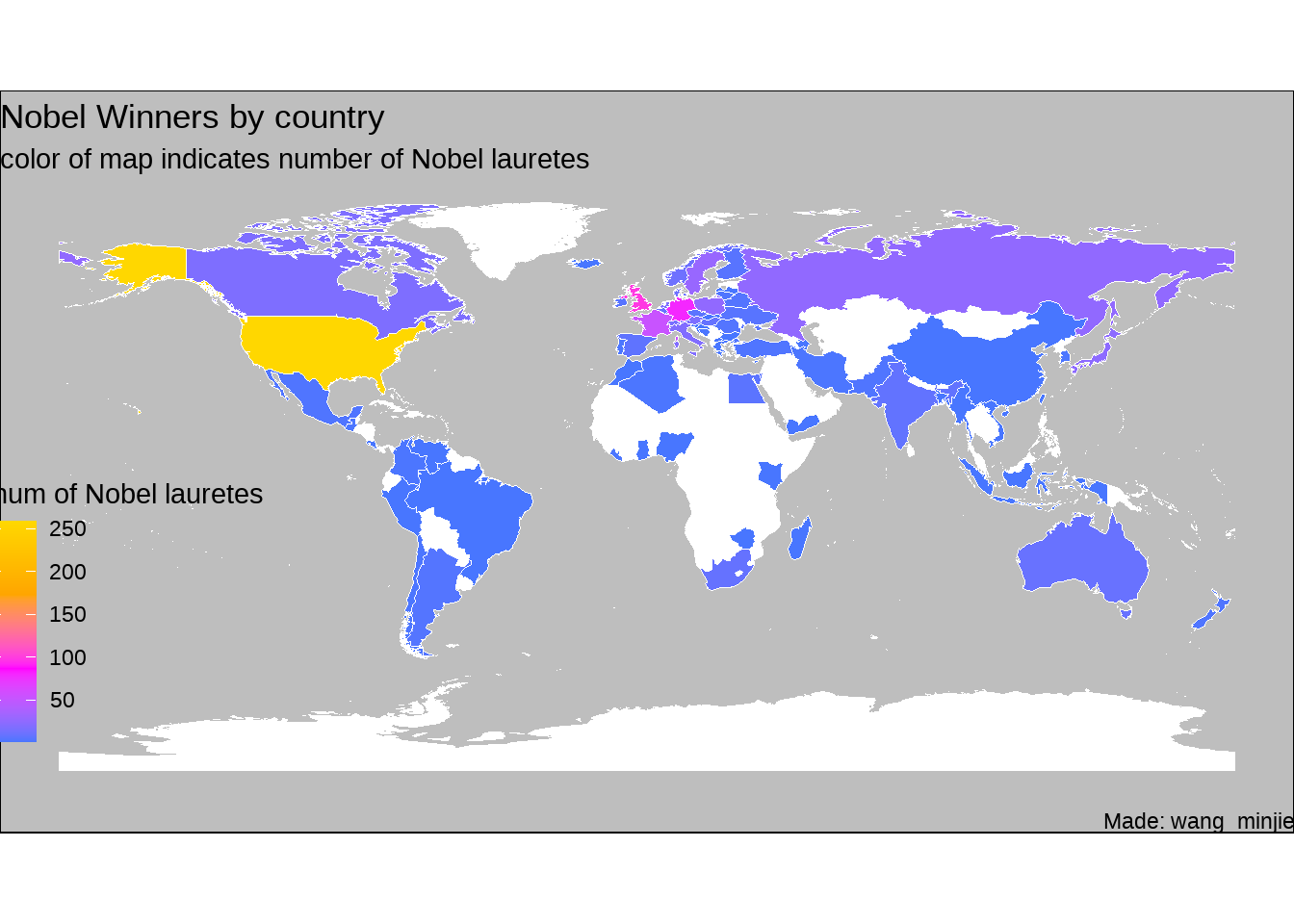
78.16 地图
library(here)
library(sf)
library(countrycode)

# countrycode('Albania', 'country.name', 'iso3c')

nobel_winners_birth_country <- nobel_winners_clean %>%
  count(birth_country) %>%
  filter(!is.na(birth_country)) %>%
  mutate(ISO3 = countrycode(birth_country,
    origin = "country.name", destination = "iso3c"
  ))


global <-
  sf::st_read("./demo_data/worldmap/TM_WORLD_BORDERS_SIMPL-0.3.shp") %>%
  st_transform(4326)
## Reading layer `TM_WORLD_BORDERS_SIMPL-0.3' from data source
## `F:\CEPS\R_for_Data_Science\demo_data\worldmap\TM_WORLD_BORDERS_SIMPL-0.3.shp'
## using driver `ESRI Shapefile'
## Simple feature collection with 246 features and 11 fields
## Geometry type: MULTIPOLYGON
## Dimension: XY
## Bounding box: xmin: -180 ymin: -90 xmax: 180 ymax: 83.57027
## Geodetic CRS: WGS 84global %>%
full_join(nobel_winners_birth_country, by = "ISO3") %>%
ggplot() +
geom_sf(aes(fill = n),
color = "white",
size = 0.1
) +
labs(
x = NULL, y = NULL,
title = "Nobel Winners by country",
subtitle = "color of map indicates number of Nobel lauretes",
fill = "num of Nobel lauretes",
caption = "Made: wang_minjie"
) +
scale_fill_gradientn(colors = c("royalblue1", "magenta", "orange", "gold"), na.value = "white") +
# scale_fill_gradient(low = "wheat1", high = "red") +
theme_void() +
theme(
legend.position = c(0.1, 0.3),
plot.background = element_rect(fill = "gray")
)
# Determine to 10 Countries
topCountries <- nobel_winners_clean %>%
  count(birth_country, sort = TRUE) %>%
  na.omit() %>%
  top_n(8)

topCountries
## # A tibble: 8 × 2
## birth_country n
## <chr> <int>
## 1 united states of america 259
## 2 united kingdom 99
## 3 germany 80
## 4 france 54
## 5 sweden 29
## 6 poland 26
## 7 russia 26
## 8 japan 24df4 <- nobel_winners_clean %>%
filter(birth_country %in% topCountries$birth_country) %>%
group_by(birth_country, category, prize_year) %>%
summarise(prizes = n()) %>%
mutate(cumPrizes = cumsum(prizes))
df4## # A tibble: 489 × 5
## # Groups: birth_country, category [47]
## birth_country category prize_year prizes cumPrizes
## <chr> <chr> <dbl> <int> <int>
## 1 france chemistry 1906 1 1
## 2 france chemistry 1912 2 3
## 3 france chemistry 1913 1 4
## 4 france chemistry 1935 2 6
## 5 france chemistry 1970 1 7
## 6 france chemistry 1987 1 8
## 7 france chemistry 2016 1 9
## 8 france economics 1983 1 1
## 9 france economics 1988 1 2
## 10 france economics 2014 1 3
## # ℹ 479 more rowslibrary(gganimate)
df4 %>%
mutate(prize_year = as.integer(prize_year)) %>%
ggplot(aes(x = birth_country, y = category, color = birth_country)) +
geom_point(aes(size = cumPrizes), alpha = 0.6) +
# geom_text(aes(label = cumPrizes)) +
scale_size_continuous(range = c(2, 30)) +
transition_reveal(prize_year) +
labs(
title = "Top 10 countries with Nobel Prize winners",
subtitle = "Year: {frame_along}",
y = "Category"
) +
theme_minimal() +
theme(
plot.title = element_text(size = 22),
axis.title = element_blank()
) +
scale_color_brewer(palette = "RdYlBu") +
theme(legend.position = "none") +
theme(plot.margin = margin(5.5, 5.5, 5.5, 5.5))
78.17 出生地和工作地不一样的占比
nobel_winners_clean %>%
  select(category, birth_country, death_country) %>%
  mutate(immigration = if_else(birth_country == death_country, 0, 1))
## # A tibble: 911 × 4
## category birth_country death_country immigration
## <chr> <chr> <chr> <dbl>
## 1 chemistry netherlands germany 1
## 2 literature france france 0
## 3 medicine poland germany 1
## 4 peace switzerland switzerland 0
## 5 peace france france 0
## 6 physics germany germany 0
## 7 chemistry germany germany 0
## 8 literature germany germany 0
## 9 medicine india united kingdom 1
## 10 peace switzerland switzerland 0
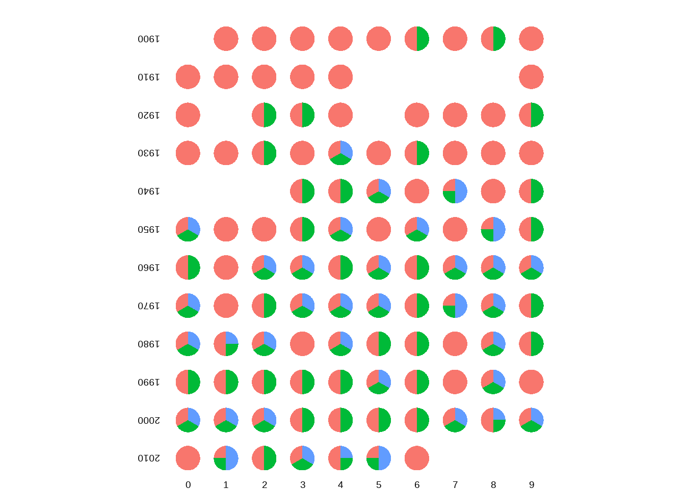
## # ℹ 901 more rows78.18 诺奖分享者
nobel_winners %>%
  filter(category == "medicine") %>%
  mutate(
    num_a = as.numeric(str_sub(prize_share, 1, 1)),
    num_b = as.numeric(str_sub(prize_share, -1)),
    share = num_a / num_b,
    year = prize_year %% 10,
    decade = 10 * (prize_year %/% 10)
  ) %>%
  group_by(prize_year) %>%
  mutate(n = row_number()) %>%
  ggplot() +
  geom_col(aes(x = "", y = share, fill = as.factor(n)),
    show.legend = FALSE
  ) +
  coord_polar("y") +
  facet_grid(decade ~ year, switch = "both") +
  labs(title = "Annual Nobel Prize sharing") +
  theme_void() +
  theme(
    plot.title = element_text(face = "bold", vjust = 8),
    strip.text.x = element_text(
      size = 7,
      margin = margin(t = 5)
    ),
    strip.text.y = element_text(
      size = 7,
      angle = 180, hjust = 1, margin = margin(r = 10)
    )
  )