第 63 章 机器学习
Rstudio工厂的 Max Kuhn 大神正主持机器学习的开发,日臻成熟了,感觉很强大啊。
63.1 数据
penguins <- read_csv("./demo_data/penguins.csv") %>%
janitor::clean_names() %>%
drop_na()
penguins %>%
head()penguins %>%
ggplot(aes(x = bill_length_mm, y = bill_depth_mm,
color = species, shape = species)
) +
geom_point()63.3 model01
model_logistic <- parsnip::logistic_reg() %>%
set_engine("glm") %>%
set_mode("classification") %>%
fit(species ~ bill_length_mm + bill_depth_mm, data = training_data)
bind_cols(
predict(model_logistic, new_data = testing_data, type = "class"),
predict(model_logistic, new_data = testing_data, type = "prob"),
testing_data
)
predict(model_logistic, new_data = testing_data) %>%
bind_cols(testing_data) %>%
count(.pred_class, species)63.7 workflow
63.7.1 使用 recipes
library(tidyverse)
library(tidymodels)
library(workflows)
penguins <- readr::read_csv("./demo_data/penguins.csv") %>%
janitor::clean_names()
split <- penguins %>%
tidyr::drop_na() %>%
rsample::initial_split(prop = 3/4)
training_data <- rsample::training(split)
testing_data <- rsample::testing(split)参考tidy modeling in R, 被预测变量在分割前,应该先处理,比如标准化。
但这里的案例,我为了偷懒,被预测变量bill_length_mm,暂时保留不变。
预测变量做标准处理。
penguins_lm <-
  parsnip::linear_reg() %>%
  #parsnip::set_engine("lm")
  parsnip::set_engine("stan")

penguins_recipe  <-
  recipes::recipe(bill_length_mm ~ bill_depth_mm + sex, data = training_data) %>%
  recipes::step_normalize(all_numeric(), -all_outcomes()) %>%
  recipes::step_dummy(all_nominal())


broom::tidy(penguins_recipe)
## # A tibble: 2 × 6
## number operation type trained skip id
## <int> <chr> <chr> <lgl> <lgl> <chr>
## 1 1 step normalize FALSE FALSE normalize_zs0oP
## 2 2 step dummy FALSE FALSE dummy_Rh8f7
penguins_recipe %>%
  recipes::prep(data = training_data) %>%  #or prep(retain = TRUE)
  recipes::juice()


penguins_recipe %>%
  recipes::prep(data = training_data) %>%
  recipes::bake(new_data = testing_data)   # recipe used in new_data


train_data <-
  penguins_recipe %>%
  recipes::prep(data = training_data) %>%
  recipes::bake(new_data = NULL)


test_data <-
  penguins_recipe %>%
  recipes::prep(data = training_data) %>%
  recipes::bake(new_data = testing_data)
63.7.2 workflows的思路更清晰
workflows的思路让模型结构更清晰。 这样prep(), bake(), and juice() 就可以省略了,只需要recipe和model,他们往往是成对出现的
wflow <-
  workflows::workflow() %>%
  workflows::add_recipe(penguins_recipe) %>%
  workflows::add_model(penguins_lm)


wflow_fit <-
  wflow %>%
  parsnip::fit(data = training_data)
wflow_fit %>%
workflows::pull_workflow_fit() %>%
broom.mixed::tidy()## # A tibble: 3 × 3
## term estimate std.error
## <chr> <dbl> <dbl>
## 1 (Intercept) 41.1 0.442
## 2 bill_depth_mm -2.33 0.297
## 3 sex_male 5.68 0.634wflow_fit %>%
workflows::pull_workflow_prepped_recipe() 先提取模型,用在 predict() 是可以的,但这样太麻烦了
wflow_fit %>%
  workflows::pull_workflow_fit() %>%
stats::predict(new_data = test_data) # note: test_data not testing_data因为,predict() 会自动的将recipes(对training_data的操作),应用到testing_data
这个不错,参考这里
penguins_pred <-
  predict(
    wflow_fit,
    new_data = testing_data %>% dplyr::select(-bill_length_mm), # note: testing_data not test_data
    type = "numeric"
  ) %>%
  dplyr::bind_cols(testing_data %>% dplyr::select(bill_length_mm))

penguins_pred
## # A tibble: 84 × 2
## .pred bill_length_mm
## <dbl> <dbl>
## 1 40.2 38.9
## 2 42.5 42.5
## 3 45.6 37.2
## 4 41.2 36.4
## 5 43.3 38.8
## 6 39.4 42.2
## 7 44.4 39.8
## 8 40.0 36.5
## 9 39.4 36
## 10 43.7 44.1
## # ℹ 74 more rowspenguins_pred %>%
ggplot(aes(x = bill_length_mm, y = .pred)) +
geom_abline(linetype = 2) +
geom_point(alpha = 0.5) +
labs(y = "Predicted ", x = "bill_length_mm") 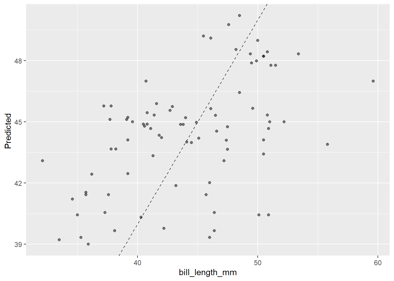
augment()具有predict()一样的功能和特性,还更简练的多
wflow_fit %>%
  augment(new_data = testing_data) %>%       # note: testing_data not test_data
  ggplot(aes(x = bill_length_mm, y = .pred)) +
  geom_abline(linetype = 2) +
  geom_point(alpha = 0.5) +
labs(y = "Predicted ", x = "bill_length_mm") 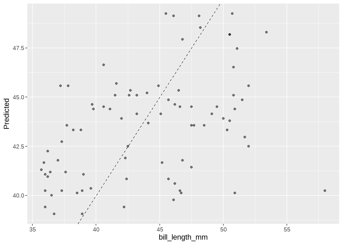
63.7.3 模型评估
参考https://www.tmwr.org/performance.html#regression-metrics
## # A tibble: 1 × 3
##   .metric .estimator .estimate
##   <chr>   <chr>          <dbl>
## 1 rmse    standard        4.94
自定义一个指标评价函数my_multi_metric,就是放一起,感觉不够tidyverse
my_multi_metric <- yardstick::metric_set(rmse, rsq, mae, ccc)

penguins_pred %>%
  my_multi_metric(truth = bill_length_mm, estimate = .pred)
## # A tibble: 4 × 3
## .metric .estimator .estimate
## <chr> <chr> <dbl>
## 1 rmse standard 4.94
## 2 rsq standard 0.179
## 3 mae standard 4.10
## 4 ccc standard 0.335